![SolidWorks Flow Simulation 2013 PDF [PDF]](https://pdfs.asia/img/200x200/solidworks-flow-simulation-2013-pdf.jpg)
29 0 26 MB
TRAINING :JULT MES
SOLIDWORKS® 2013
rorks Flow Simulation
ENG
SystematiCS Lim1ted 4 Raoul Wallenberg St. Tel Aviv, 69719 II
Systematics
111111/ l
:J I
SolidWorks® 2013 SolidWorks Flow Simulation
r
n ("'")
Dassault Systemes SolidWorks Corporation 175 Wyman Street Waltham, Massachusetts 02451 USA
0 1995-2012, Dassault Systemes SolidWorks Corporation, a Dassault Systemes S.A. company, 175 Wyman Street, Waltham, MA. 02451 USA. All rights reserved. The infonnation and the software discussed in this document are subject to change without notice and are not commitments by Dassault Systemes Solid Works Corporation (DS SolidWorks). No material may be reproduced or transmitted in any fonn or by any means, electronically or manually, for any purpose without the express written pennission of DS SolidWorks. The software discussed in this document is furnished under a license and may be used or copied only in accordance with the tenns of the license. All warranties given by DS Solid Works as to the software and documentation are set forth in the license agreement, and nothing stated in, or implied by, this document or its contents shall be considered or deemed a modification or amendment of any tenns, including warranties, in the license agreement. (C)
Patent Notices
Solid Works® 3D mechanical CAD software is protected by U.S. Patents 5,815,154; 6,219,049; 6,219,055; 6,611,725; 6,844,877; 6,898,560; 6,906,712; 7,079,990; 7,477,262; 7,558,705; 7,571,079; 7,590,497; 7,643,027; 7,672,822; 7,688,318; 7,694,238; 7,853,940; 8,305,376 and foreign patents, (e.g., EP 1,116,190 B I and JP 3,517,643). eDrawings® software is protected by U.S. Patent 7,184,044; U.S. Patent 7,502,027; and Canadian Patent 2,318,706. U.S. and foreign patents pending. Trademarks and Product Names for SolidWorks Products and Services Solid Works, 3D PartStream.NET, 3D ContentCentral, eDrawings, and the eDrawings logo are registered trademarks and FeatureManager is a jointly owned registered trademark of DS Solid Works. CircuitWorks, FloXpress, Photo Works, ToiAnalyst, and XchangeWorks are trademarks of DS SolidWorks. Feature Works is a registered trademark of Geometric Ltd. Solid Works 2013, Solid Works Enterprise PDM, SolidWorks Workgroup PDM, Solid Works Simulation, Solid Works Flow Simulation, eDrawings, eDrawings Professional, and Solid Works Sustainability are product names of DS Solid Works. Other brand or product names are trademarks or registered trademarks of their respective holders. COMMERCIAL COMPUTER SOFTWARE PROPRIETARY The Software is a "commercial item" as that tenn is defined at 48 C.F.R. 2.10 I (OCT 1995), consisting of "commercial computer software" and "commercial software documentation" as such tenns are used in 48 C.F.R. 12.212 (SEPT 1995) and is provided to the U.S. Government (a) for acquisition by or on behalf of civilian agencies, consistent with the policy set forth in 48 C.F.R. 12.212; or (b) for acquisition by or on behalf of units of the department of Defense, consistent with the policies set forth in 48 C.F.R. 227.7202-1 (JUN 1995) and 227.7202-4 (JUN 1995). In the event that you receive a request from any agency of the U.S. government to provide Software with rights beyond those set forth above, you will notifY DS Solid Works of the scope of the request and DS Solid Works will have five (5) business days to, in its sole discretion, accept or reject such request. Contractor/Manufacturer: Dassault Systemes Solid Works Corporation, 175 Wyman Street, Waltham, Massachusetts 02451 USA.
Copyright Notices for SolidWorks Standard, Premium, Professional, and Education Products Portions of this software «:11986-2012 Siemens Product Lifecycle Management Software Inc. All rights reserved. This work contains the following software owned by Siemens Industry Software Limited: D-CubedT" 20 DCM © 2012. Siemens Industry Software Limited. All rights reserved. D-CubedT" 30 DCM © 2012. Siemens Industry Software Limited. All rights reserved. D-CubedTM PGM © 2012. Siemens Industry Software Limited. All rights reserved. D-Cubed™ COM (C) 2012. Siemens Industry Software Limited. All rights reserved. D-Cubed™ AEM © 2012. Siemens Industry Software Limited. All rights reserved. Portions of this software© 1998-2012 Geometric Ltd. Portions of this software© 1996-2012 Microsoft Corporation. All rights reserved. Portions of this software incorporate PhysXTM by NVIDIA 2006-2010. Portions of this software (C) 2001-2012 Luxology, LLC. All rights reserved, patents pending. Portions of this software© 2007-20 II Drive Works Ltd. Copyright 1984-20 I 0 Adobe Systems Inc. and its licensors. All rights reserved. Protected by U.S. Patents 5,929,866; 5,943,063; 6,289,364; 6,563,502; 6,639,593; 6,754,382; patents pending. Adobe, the Adobe logo, Acrobat, the Adobe PDF logo, Distiller and Reader are registered trademarks or trademarks of Adobe Systems Inc. in the U.S. and other countries. For more DS Solid Works copyright infonnation, see Help> About Solid Works. Copyright Notices for SolidWorks Simulation Products Portions of this software© 2008 Solversoft Corporation. PCGLSS «:! 1992-20 I 0 Computational Applications and System Integration, Inc. All rights reserved. Copyright Notices for Enterprise PDM Product
Outside In® Viewer Technology, © 1992-2012 Oracle © 20 II, Microsoft Corporation. All rights reserved. Copyright Notices for eDrawings Products Portions of this software© 2000-2012 Tech Soft 3D. Portions of this software© 1995-1998 Jean-Loup Gailly and Mark Adler. Portions of this software© 1998-200 I 3Dconnexion. Portions of this software© 1998-2012 Open Design Alliance. All rights reserved. Portions of this software© 1995-2010 Spatial Corporation. This software is based in part on the work of the Independent JPEG Group.
Portions of eDrawings® for iPad® © 1996-1999 Silicon Graphics Systems, Inc. Portions of eDrawings® for iPad® © 2003-2005 Apple Computer Inc.
Document Number: PMT1343-ENG
u
u u
u u u
u u
r r
Contents
r
Introduction About This Course .................. . .. . ......... ... ...... 2 Prerequisites ...................... .. .......... . ....... 2 Course Design Philosophy ....... . .. ..... .......... ... ... 2 Using this Book ....................................... 2 Lessons ... ........................................... 2 About the Training Files ................................. 3 Windows® 7 ........ . ........... . ..................... 3 Conventions Used in this Book ..... ... ................... 3 Use of Color ....... . .................................. 3
Lesson 1: Creating a SolidWorks Flow Simulation Project Objectives ............................................... 5 Case Study: Manifold Assembly ................... .... ...... 6 Problem Description ................. .. ........... ... ...... 6 Stages in the Process ..... ... .. .... .... . ....... . ... . ... .. 6 Model Preparation ................... .... .................. 7 Internal Flow Analysis .................................. 7 External Flow Analysis .................................. 7 Manifold Analysis .... ..... ........ ..... ................ 7 Lids ................................................. 8 Lid Thickness ......................................... 9 Manual Lid Creation .................................... 9 Adding a Lid to a Part File ......... ..... ................. 9 Adding a Lid to an Assembly File ........................ 10 Checking the Geometry ................................ I I Internal Fluid Volume .............. .. .................. 13
Contents
SolidWorks 2013
Invalid Contacts ...................................... 13 Project Wizard ....................................... 17 Reference Axis ....................................... 20 Exclude Cavities Without Flow Conditions ................. 20 Adiabatic Wall ....................................... 22 Roughness ........................................... 22 Result Resolution ..................................... 24 Computational Domain ................................. 25 Load Results Option ................................... 30 Monitoring the Solver. ... ... ... .... .. .................. 31 Goal Plot Window .. . . ........... . ....... ............. 31 Warning Messages ................. .. .... . ..... . ..... . 32 Post-processing .......................................... 34 Scaling the Limits of the Legend ......................... 36 Changing Legend Settings .... . ........... .. ........... . 3 7 Discussion .............................................. 46 Summary ... .. .................................. ... ..... 46
Lesson 2: Meshing
LJ u u
\....,)
u
u Objectives .............................................. 47 Case Study: Chemistry Hood .............. ... ...... . ... ... . 48 Project Description ....................................... 48 Computational Mesh ...................................... 51 Basic Mesh ... ... ....... ............. .. .... .... .. ...... . 51 Initial Mesh .. ................ .... .... .. .... ... .......... 52 Geometry Resolution ...... . ... .... .......... ... .... . ..... 52 Optimize Thin Wall Resolution ............................. 53 Result Resolution/Level of Initial Mesh ... . ............ . ..... . 56 Switching Off Automatic Mesh Definition ................. 57 Cell Types ................ ... ... .... ........... .... .. 58 Basic Mesh .... . ..... . ............................... 58 Solid/Fluid Interface ................................... 58 Refining Cells .............. .. .... . .................. . 58 Narrow Channels ..................................... 58 Advanced Narrow Channel Refinement .................... 58 Control Planes ..... .. .... . ............................... 61 Results ................................................. 65 Summary ............................................... 66 Exercise I: Square Ducting ................................. 67 Exercise 2: Thin Walled Box . ... ... ........... . ..... . ..... . 75 Exercise 3: Heat Sink ..................................... 81 Exercise 4: Meshing Valve Assembly ........................ 87 Boundary Conditions ..... ... ..... .. ..... . ............. 87
u LJ u
LJ ._)
u \_j
u ii
L..l
SolidWorks 2013
r
Contents
Lesson 3: Thermal Analysis Objectives ..... . ... .. . . . . ... . . . . . ... . . . . . ... . .... . ...... 89 Case Study: Electronics Enclosure .... . .............. .. .. . . . . 90 Project Description .......... . . . . .. ...................... . 90 Fans ......................... . . . .................... . . . 96 Fan Curves .............. . .................... . . .... . 96 Perforated Plates ......................................... 98 Free Area Ratio ...... .... . . ....... . ........ . .. ... . ... I 00 Discussion .. . .. .. ... .......... ... . .. . . . . .. ... . . ........ I 02 Summary ........ . . . .......... . . . .. . .... . . ... . . . . ...... I 02 Exercise 5: Materials with Orthotropic Thermal Conductivity .... 103
r
r r
r
Lesson 4: External Transient Analysis Objectives . ............. .. . ......... . . .......... . . . . ... Case Study: Flow Around a Cylinder ..... .............. ... .. Problem Description ....... ...... . . . . ............... . . . . . Stages in the Process ...... ..... . .. ................... . Reynolds Number ......... .... . ... ................. ..... External Flow ......... ......... . . . .... .......... . . .. . .. Transient Analysis .. .. ......... .... . ... . . . . .. . ....... . . . Turbulence Intensity .. . . . . .... . ..... . .. .. . . . . .. . ..... .. . . Solution Adaptive Mesh Refinement ..... . . . .. . . ...... .... .. Two Dimensional Flow ..... . . .. ......... . ... ... . . . ... ... . Computational Domain. . . . . . . . . . . . . . . . . . . . . . . . . . . . . . . . . . . Calculation Control Options ... . ... . . ................ ...... Finish . ................ ..... ..................... .. Refinement . . . . . . . . . . . . . . . . . . . . . . . . . . . . . . . . . . . . . . . . . Saving . . ............ .. . . . . .. .. ................ ..... Advanced ............ . ... ...... ........... . . ....... Drag Equation ........ .. . . . . . .. . .... .... . ........... . Unsteady Vortex Shedding .. . .. .. . . . . .. .. . . . . .. . . . . ... . Time Animation .. . ... . . ... ... . ... . . ... . ... . . . . ... . .... . Discussion . . . . . ... . ... . . . . .. . . .. . ... . . . . ... . ... . ... ... . Summary . . . .. . ...... . . . . . ..... . .. . .... .. ..... ... ... . .. Exercise 6: Electronics Cooling .. . . .... . ............ . . .... .
Ill 112 113 113 113 113 115 115 116 116 117 117 117 I 18 118 118 120 122 123 126 126 127
r
r
Iii
u Contents
SolidWorks 2013
Lesson 5: Conjugate Heat Transfer Objectives ............................................. Case Study: Heated Cold Plate ............................. Project Description ...................................... Stages in the Process. . . . . . . . . . . . . . . . . . . . . . . . . . . . . . . . . . Conjugate Heat Transfer .................................. Real Gases .................................. . .......... Goals Plot in the Solver Window ........................ Summary .............................................. Exercise 7: Heat Exchanger with Multiple Fluids .............. Lesson 6: EFDZooming Objectives ............................................. Case Study: Electronics Enclosure .......................... Project Description ...................................... EFD Zooming .......................................... EFD Zooming- Computational Domain .................. Summary .............................................. Lesson 7: Porous Media Objectives ............................................. Case Study: Catalytic Converter ............................ Problem Description ..................................... Stages in the Process .................................. Porous Media .......................................... Porosity . . . . . . . . . . . . . . . . . . . . . . . . . . . . . . . . . . . . . . . . . . . . Permeability Type .................................... Resistance .......................................... Dummy Bodies ...................................... Design Modification ..................................... Discussion ............................................. Summary .............................................. Exercise 8: Channel Flow ................................. Lesson 8: Rotating Reference Frames Objectives ............................................. Rotating Reference Frame ................................ Case Study: Fan Assembly ................................ Problem Description ..................................... Stages in the Process .................................. Summary ..............................................
139 140 140 140 141 141 145 147 148
153 154 154 154 157 164
u
u L.l
u u u
165 166 166 166 168 168 168 168 170 174 178 178 179
187 188 188 188 189 195
w u
u
u 1.......1
'--'
u
u iv
.._;
SolidWorks 2013
Contents
n n
Lesson 9: Parametric Study
Objectives ............................................. 197 Case Study: Piston Valve ................................. 198 Problem Description ..................................... 198 Stages in the Process .................................. 198 Parametric Analysis ..................................... 199 Steady State Analysis .................................... 199 Parametric study ..................................... 202 Part I: Goal Optimization ................................. 203 Input Variable Types ................................. 204 Target Value Dependance Types ........................ 205 Output Variable Initial Values .......................... 205 Running Optimization Study ........................... 206 Part 2: Design Scenario ................................... 209 Summary .............................................. 211 Exercise 9: Variable Geometry Dependent Solution ............ 212 Boundary Conditions ................................. 213
r
r n r
r
Lesson 10: Cavitation
n
r
n
Objectives ............................................. Case Study: Cone Valve .................................. Problem Description ..................................... Cavitation ............................................. Discussion ............................................. Summary ..............................................
215 216 216 216 220 220
Objectives ............................................. Relative Humidity ....................................... Case Study: Cook House ................................. Problem Description ..................................... Summary ..............................................
221 222 222 222 229
Objectives ............................................. Case Study: Hurricane Generator ........................... Problem Description ..................................... Particle Trajectories - Overview ............................ Particle Study- Physical Settings ........................ Particle Study- Wall Condition ......................... Summary .............................................. Exercise I 0: Uniform Flow Stream .........................
231 232 232 232 238 238 239 240
Lesson 11: --..,Relative Humidity
Lesson 12: Particle Trajectory
r
n r
v
Contents
i
SolidWorks 2013
Lesson 13: Supersonic Flow Objectives .................................... . ........ Supersonic Flow ........................................ Case Study: Conical Body ................................ Problem Description ..................................... Drag Coefficient ..... .. .............................. Shock Waves ........................................ Discussion ............................................. Summary ..............................................
245 246 246 246 24 7 251 252 252
Objectives ........... .. .......... . ........... ... ....... Case Study: Billboard .................................... Problem Description ..................................... Summary ....................................... .. .....
253 254 254 259
w
Lesson 14: FEA Load Transfer \....)
u
u
u
vi
r r r r
r r r
r
r
r.
Introduction
('
(j
r
n r
r
r
r
r
r r
n
0
r r r
(\
r r r
r r
r r (j
1
Introduction
About This Course
SolidWorks 2013
The goal of this course is to teach you how to set up, run and view results of a fluid flow and/or heat transfer analysis using SolidWorks and the Standard version of Solid Works Flow Simulation mechanical design automation software. It is impractical to cover every type of computational fluid dynamics (CFD) problem in the SolidWorks Flow Simulation software and still have the course be a reasonable length. Therefore, the focus of this course is on the fundamental skills and concepts central to successfully performing a CFD analysis. You should view the training course manual as a supplement to, not a replacement for, the system documentation and on-line help. Once you have developed a good foundation in basic skills, you can refer to the on-line help for information on less frequently used command options.
Prerequisites
Students attending this course are expected to have: • • • •
Course Design Philosophy
Mechanical design experience. Completed the course SolidWorks Essentials. Basic understanding in the field of fluid flow and heat transfer. Experience with Windows operating system.
This course is designed around a process- or task-based approach to training. A process-based training course emphasizes the processes and procedures you follow to complete a particular task. By utilizing case studies to illustrate these processes, you learn the necessary commands, options and menus in the context of completing a task.
Course Length
The recommended minimum length of this course is 2 days.
Using this Book
This training manual is intended to be used in a classroom environment under the guidance of an experienced Solid Works Flow Simulation instructor. It is not intended to be a self-paced tutorial.
Lessons
The lessons give you the opportunity to apply and practice the material in front of an instructor so questions can be asked and answered during each lesson.
u u
u
u u
u L) \...)
u ...__)
u
w :__)
u u Lj
u \_)
u ~
u u 2
u
Introduction
SolidWorks 2013
r About the Training Files
r ('\
A complete set of the various files used throughout this course can be downloaded from the SolidWorks website, www.solidworks.com. Click on the link for Support, then Training, then Training Files, then SolidWorks Simulation Training Files. Select the link for the desired file set. There may be more than one version of each file set available. Direct URL:
0
www.solidworks.com/trainingfilessimulation
r
The files are supplied in signed, self-extracting executable packages.
r r r
The files are organized by lesson number. The Case Study folder within each lesson contains the files your instructor uses while presenting the lessons. The Exercises folder contains any files that are required for doing the laboratory exercises. Windows®7
The screen shots in this manual were made using the SolidWorks and SolidWorks Flow Simulation software running on Windows® 7. If you are running on a different version of Windows, you may notice differences in the appearance of the menus and windows. These differences do not affect the performance of the software.
Conventions Used in this Book
This manual uses the following typographic conventions: Convention Bold Sans Serif
SolidWorks Flow Simulation commands and options appear in this style. For example, SolidWorks Flow Simulation, Project, Wizard means choose the Wizard option from the SolidWorks Flow Simulation, Project
(1
menu.
n
Typewriter
r 17 Do this step
n Use of Color
r
Meaning
Feature names and file names appear in this style. For example, Heat Source. Double lines precede and follow sections of the procedures. This provides separation between the steps of the procedure and large blocks of explanatory text. The steps themselves are numbered in sans serif bold.
The SolidWorks and SolidWorks Flow Simulation user interface make extensive use of color to highlight selected geometry and to provide you with visual feedback. This greatly increases the intuitiveness and ease of use of the SolidWorks Flow Simulation software. To take maximum advantage of this, the training manuals are printed in full color.
3
u Introduction
SolidWorks 2013
'\.....)
u
w u ._)
u .._)
\.._)
u u u .._)
0 ......._, .._) I.....J
'--' ...__)
'-'
w u
Li
u u .._)
u ....) ..__) .._)
.___)
w u ...__) 4
u \. .J
r
Lesson 1 Creating a SolidWorks Flow Simulation Project
Objectives
r: n
r
r
Upon successful completion of this lesson, you will be able to: •
Understand the model preparations required for a Flow Simulation Project.
•
Create simple lids.
•
Check the geometry for invalid contacts.
•
Calculate the internal volume.
•
Create a Solid Works Flow Simulation Project using the Project Wizard.
•
Apply flow boundary conditions.
•
Apply Goals.
•
Run an analysis.
•
Use the Solver Monitor window.
•
View the results.
5
Lesson 1
SolidWorks 2013
Creating a SolidWorks Flow Simulation Project
Case Study: Manifold Assembly Problem Description
Stages in the Process
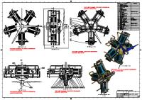
In this lesson, we will learn how to set up a SolidWorks Flow Simulation project using the Wizard. Prior to setting up our project, we will learn how to properly prepare our model for the analysis. We will run the simulation and learn how to interpret the results. In addition, we will see the many options available when post-processing the results. Air enters an intake manifold assembly at 0.05 m3/s and flows out through the six openings as seen in the figure. The common goal of intake manifold design is even distribution of the combustion mixture to the piston heads. This will insure optimum engine efficiency. We will keep this in mind when analyzing our intake assembly.
u LJ
w
u u ..1..
The objective of this lesson is to introduce the complete set up of a SolidWorks Flow Simulation project within SolidWorks, from model preparation to post-processing. Study goals will be defined and discussed. In addition, the results will be post-processed using the various options in SolidWorks Flow Simulation.
\......)
•
LJ
Prepare model for analysis. Use the Lids tool to close the model in preparation for an internal analysis. The Check Geometry command will be used to make sure that your model is ready for a flow simulation.
•
Set up flow simulation. Use the Wizard to set up the flow simulation project.
•
Apply boundary conditions. Boundary conditions are applied to inlets and outlets.
•
Declare calculation goals. Goals can be defined that are special parameters that the user will have information for after the analysis is run.
•
Run the analysis.
•
Post-process the results. The results can be processed using many available options in SolidWorks Flow Simulation.
L.)
w u u \......)
6
r
SolidWorks 2013
Lesson 1 Creating a SolidWorks Flow Simulation Project
1
Open SolidWorks.
2
SolidWorks Flow Simulation Add-Ins. Once installed, SolidWorks Flow Simulation can be activated inside SolidWorks using the Tools, Add-Ins menu.
r
Check SolidWorks Flow Simulation to use this Add-In.
r
Click OK.
r
r r.
3
Model Preparation
In any static analysis, it is often necessary to modify the Solid Works geometry to allow the simulation to run. The same is true in flow simulations. SolidWorks Flow Simulation groups flow analysis into two separate categories, internal analysis and external analysis. Before beginning model preparations, it is necessary to ask yourself which type of analysis you wish to perform.
Internal Flow Analysis
Internal flow analysis involves fluid flow bounded by outer solid surfaces, e.g. flows inside pipes, tanks, HVAC systems, etc. Internal flows are confined inside the SolidWorks geometry. For internal flows the fluid enters a model through the inlets and exits the model through the outlets with the exception of some natural convection problems that have no openings.
r
n n
"r r
r
To perform an Internal flow analysis, the SolidWorks model must be fully closed (no openings) using lids. The SolidWorks Flow Simulation, Tools, Check Geometry command tool can be used to ensure that the model is fully closed.
r
n
r
Open Assembly. Open Coletor from the LessonOl \Case Study folder.
n
External flow analysis involves a solid model which is fully surrounded by the flow, e.g., flows over aircraft, automobiles, buildings, etc. The fluid flow is not bounded by an outer solid surface, but bounded only by the Computational Domain boundaries and does not require a lid unless the application involves a flow source (such as a fan).
r
If both internal and external analysis is required simultaneously, e.g., flows over and through a building, the analysis is treated as an External analysis in SolidWorks Flow Simulation.
n n
r n r
n
r. n
n
External Flow Analysis
Manifold Analysis
Now that we know the difference between internal and external analysis, we can characterize our manifold analysis as internal. We will only study the flow on the inside of the manifold assembly and are not concerned with any flows around the body. As mentioned previously, to perform an internal flow analysis, the SolidWorks model must be fully closed using Lids.
7
SolidWorks 2013
Lesson 1 Creating a SolidWorks Flow Simulation Project
Lids are used in internal flow analysis. In this type of analysis, all openings within a model must be covered using the SolidWorks "lids" features. The surfaces of the lids (which contact the fluid) are used to apply boundary conditions which introduce a mass flow rate, volume flow rate, static /total pressure, of Fan condition within a fluid volume.
Lids
Note
Situations that do not require the use of lids include external analysis that measure flow over bodies such as: cars, planes, buildings, ... etc. In addition, lids are not used in natural convection problems.
Introducing: Create Lids
The Create Lids tool automatically creates lids for all openings in the selected planar surface of the model. This tool is available for both part and assembly files. The lids are necessary for an internal analysis (problems such as flow through a ball valve or pipe).
Where to Find It
• • • 4
u 0
CommandManager: Flow Simulation > Create lids ~ Menu: Flow Simulation, Tools, Create lids Flow Simulation Main toolbar: Create Lids ~
Create a lid on the inlet face. Under SolidWorks Flow Simulation, Tools, select Create lids.
Select the annular face defining the plane of the inlet that should be closed by the lid.
LJ
In the Create Lids PropertyManager, select Adjust Thickness and enter 1mm as the Thickness. Click OK.
You' ll notice that a new part called LID! gets created in the FeatureManager design tree. The part is a blind extrusion from the selected planar face into the opening with a distance that was specified as the Thickness.
u
8
Lesson 1
SolidWorks 2013
Creating a SolidWorks Flow Simulation Project
n
r
Note
Multiple planar faces can be selected using the Create lids tool. If the user is working with an assembly, new parts named LIDl, LID2 ... will be created. If the user is working with a single part, new LIDl, LID2 .. .features will be created.
Tip
It is good practice to rename your lids when working in an assembly. This can avoid problems with multiple assemblies with lids open at the same time.
Lid Thickness
If necessary, the thickness of the lid can be adjusted by clicking the Adjust Thickness icon and input the value in the Thickness box (as done in the previous step). The thickness of an external lid for an internal analysis is usually not important for the analysis. However, the lid should not be so thick that the flow pattern is affected downstream in some way. If this is both an external and internal analysis then creating a lid that is too thin will cause the number of cells to be very high. For most cases the lid thickness could be the same thickness used to create the neighboring walls.
r
r
r (\
r
Manual Lid Creation
The Create lids tool cannot be used if there are no planar faces to use as references. In this instance, the user must create the lids manually by creating lid parts or features .
Adding a Lid to a Part File
•
Click on the surface adjacent to where you would like to add the lid and open a sketch.
•
Select the inside edge(s) and select Sketch Tools, Convert Entities. Insert, Boss/Base, Extrude and select the Mid Plane option.
r
• Note
r
Selecting the Mid Plane option is very important. The Blind option would create an invalid contact (disjointed body) between the lid and the body. SolidWorks Flow Simulation is unable to apply boundary conditions onto a surface when there is an invalid contact. Blind extrus1on
Correct Lid Creation
In-correct Lid Creation
9
Lesson 1
SolidWorks 2013
Creating a SolidWorks Flow Simulation Project
Adding a Lid to an Assembly File
There are several ways to create lids within a SolidWorks assembly file. The following steps outline one of these recommended ways. • • • • •
Note
Within the SolidWorks assembly mode go to Insert, Component, New Part. Type in a name for the part file (many people use Inlet lid or Outlet lid). Click OK. Select the surface adjacent to where you would like to add the lid. Select the inside edge(s) and select Sketch Tools, Convert Entities. Insert, Boss/Base, Extrude and select the Mid Plane option.
It's usually a good idea to create the lids as a part file within an assembly especially if your analysis involves heat transfer. These lids can then be assigned a different material, such as an insulator so that the lid does not affect the heat transfer analysis. 5
Remaining lids. Create the remaining lids on the outlet faces using the manual lid creation method described above. Use a Mid Plane extrusion of2mm.
u u
Note
We could have used the Create Lids tool to create the remaining lids, however the tool would have closed all of the openings on the selected face, therefore closing the bolt holes. This is not necessary, and this also gives us the opportunity to practice manual lid creation.
u 10
Lesson 1
SolidWorks 2013
Creating a SolldWorks Flow Simulation Project
Discussion
When creating lids before the analysis, keep in mind that they have two purposes; closing off any openings and allowing for solid geometry on which boundary conditions (i.e. static pressure, mass flow rate, etc.) are defined. In this model, we could have used a single part to close off all six outlet ports as shown in the figure. This type of lid would not be applicable if we required different boundary conditions on each outlet. In addition, this lid is inappropriate because to evaluate the design, we require information about the flow through each individual outlet (remember, a well designed manifold will distribute the combustion mixture evenly). We will see that this type of lid will make it more difficult to obtain the information about each port.
Checking the Geometry
The SolidWorks model must be checked to determine if there are any problems with the geometry that may cause problems meshing the body and fluid regions.
n
There are two main reasons that prevent meshing of the solid and fluid bodies. •
•
Note
Openings in the geometry that prevent SolidWorks from fully defining a fully closed internal volume. This is for an internal analysis only. Invalid contacts exist between parts in an assembly. (An invalid contact is defined as a line or point contact between part files.) These will be discussed later in the lesson.
Invalid contacts affect both internal and external analysis.
11
Lesson 1
SolidWorks 2013
\.....)
Creating a SolidWorks Flow Simulation Project
Introducing: Check Geometry
A SolidWorks Flow Simulation tool, called Check Geometry, allows users to check the SolidWorks geometry. This tool also allows you to check bodies for possible geometry problems (e.g., tangent contact) that cause SolidWorks Flow Simulation to create an inadequate mesh.
'~~ C~eck Geometrv- -I
\....) '"'rn ~·,..;l Check Geometry ~ Menu: Flow Simulation, Tools, Check Geometry Flow Simulation Main toolbar: Check Geometry ~
Check for invalid fluid geometry. From the Flow Simulation menu choose: Tools, Check Geometry. Keep all assembly components selected. Click Check.
~· Check Geom~y ___;,_;r
)C
..
Sta... •
-
•
J
lil ~ SWldomaons ~ eo..nda
ill'
Goo~>
~ loco!.....,. Meshes
8 ~ R...As
ji$. Mesh
u
~ Co.tl'tots
{)>
S..focel'tots
~ Jsoswfoces AowTra;ectories
»
u
Click Next.
u '.._) 18
lesson 1
SolidWorks 2013
Creating a SolidWorks Flow Simulation Project
14 Select units. Wu.rd · Untt Sys~ Unlaystenr
Sjnlem
Palh
Convner
ll.med f'le{).med f'le{).med f'l&{).med
CGS 1""'11·•1 FPS lfi.J>-•1 IPS [....,_•1 NMMI""'11•1
USA
f'le{).med
USA
51 lm·ko·•lln> ~ Ddoult q : Praject 1
Unrts••• Component Control
~
JniiiiiMesh... Clkullbon Control Opoons...
lluplly All Collouts 0 ~~ ~~b------~--------~
Expand the options under Input Data within the SolidWorks Flow Simulation analysis tree. The SolidWorks Flow Simulation analysis tree is used to define additional analysis settings for the project. The Computational Domain, shown as a wireframe box enveloping the model, is used to visualize the volume being analyzed.
24
Lesson 1
SolidWorks 2013
Creating a SolidWorks Flow Simulation Project
Computational Domain
The Computational Domain is defined as a volume fixed with respect to a coordinate system within a fluid flow field. Although the fluid moves into and out of the computational domain, the computational domain itself remains fixed in space. SolidWorks Flow Simulation analyzes the model geometry and automatically generates a Computational Domain in the shape of a rectangular prism enclosing the model. The computational domain's boundary planes are orthogonal to the model's Global Coordinate System axes. For external flows, the computational domain's boundary planes are automatically distanced from the model capturing the fluid space around the model. However, for internal flows, the computational domain's boundary planes automatically envelop the model walls only.
Introducing: Boundary Conditions
A boundary condition is required to describe where the fluid enters or exits the system (Computation Domain) and can be set as a Pressure, Mass Flow, Volume Flow or Velocity. Boundary conditions can also specify parameters of a wall such as ideal, stationary, or rotating.
Where to Find It
• •
Shortcut Menu: Right-click Boundary Conditions in the Flow Simulation analysis tree and click Insert Boundary Condition CommandManager: Flow Simulation > Boundary Conditions
•
Menu: Flow Simulation, Insert, Boundary Condition
~
21 Insert boundary condition. In the SolidWorks Flow Simulation analysis tree, under Input Data, rightclick Boundary Conditions and select Insert Boundary Condition. Select the inside surface of the SolidWorks feature representing the inlet, as shown in the figure. Note
To access the inner face, right-click the outer face on the lid and click Select Other. In the Select Other window, cycle through the faces by moving the pointer to highlight each face dynamically in the solid geometry.
n
r
2.5
SolidWorks 2013
Lesson 1 Creating a SolidWorks Flow Simulation Project
22 Set up the boundary condition. In the Boundary Conditions PropertyManager, under Type, select the Flow openings button
*
[B . Still under Type, select Inlet Volume Flow. Under Flow Parameters, click the Normal to face button fB and enter 0.05 m 3/s.
I
~ ,f.. ~===~== Face Coorcinale Sy;tem
Rer.r""""""' ~~.--~
Click OK. The new Inlet Volume Flow! item appears in the SolidWorks Flow Simulation analysis tree under Boundary Conditions. Solid Works Flow Simulation will apply a 0.05 m3 of air per second across the inlet area, nonnal to the selected face.
Inlet Velocity IrietMachl't.mber
OJIJetMa=:sRow OJIIetVolu'ne:Aow OUIJetVekxity
Q
e
O.ll5m"'3/•
;
1£)
IB
Untoon
L.)
~ MJy dovelopod ftow
_ ___J
Note
Since the volume flow rate is required as an output at each outlet, a pressure condition should be used to identify the outlet condition. If the pressure is not known at the outlet of each port, an ambient static pressure condition can be used as the boundary condition across each outlet face for this analysis. 23 Insert boundary condition.
In the SolidWorks Flow Simulation analysis tree, under Input Data, right-click the Boundary Conditions icon and select Insert Boundary Condition.
Select the inner face of one of the outlet ports.
u
\_)
u 26
SolidWorks 2013
Lesson 1 Creating a SolidWorks Flow Simulation Project
24 Set up the boundary condition. In the Boundary Conditions window, under Type, select the Pressure openings button ~ · Still under Type, select Static Pressure. Click OK to accept the default ambient values . The new Static Pressure l item appears in the SolidWorks Flow Simulation analysis tree.
~
P
101325Pa
T
293.2K
............... ,. ;
~
25 Create additional outlet boundary conditions. Each outlet port should have a static pressure boundary condition assigned to the inside outlet lid surface. Create five additional static pressure boundary conditions for the remaining five outlets. Introducing: Engineering Goals
n n
i
-~ ~ II
SolidWorks Flow Simulation contains built-in criteria to stop the solution process. However, it is best to use your own criterion by using what SolidWorks Flow Simulation calls Goals. You can specify the Goals as physical parameters at areas of interest in the project, so that their convergence can be considered as obtaining a steady state solution from the engineering viewpoint. Engineering goals are user specified parameters of interest, which the user can display while the solver is running and obtain information about after convergence is reached. Goals can be set throughout the entire domain (Global Goal), in a selected area (Surface Goal, Point Goal), or within a selected volume (Volume Goal). Furthennore, SolidWorks Flow Simulation can consider the average, minimum or maximum value when examining goals.
27
Lesson 1
SolidWorks 2013
Creating a SolidWorks Flow Simulation Project
In addition, you can also define an Equation Goal, which is a goal defined by an expression (basic mathematical functions) using the existing goals as variables. This allows you to calculate a parameter of interest (e.g., pressure drop) and keeps this infonnation in the project for later reference. There are five different types of goals that can be defined in SolidWorks Flow Simulation:
Where to Find It
Global Goal Surface Goal Equation Goal
•
Shortcut Menu: Right-click Goals in the Flow Simulation analysis tree and click Insert Goals CommandManager: Flow Simulation > Flow Simulation Features • > Goals Menu: Flow Simulation, Insert, Goals
• • Use in Instructions
.__)
• • •
• •
Point Goal Volume Goal
Choose the type of goal you want to define. 26 Insert surface goal. In the SolidWorks Flow Simulation analysis tree, right-click Goals, and select Insert Surface Goals.
Pn>JOUDt+.l
l!l Fecr:CUD11: 1
Goals InletSG-FiowRate I Ol. to automatically move the cutting plane (Top plane in our example) through the mode and view how the plotted quantity varies.
r
Close the animation toolbar.
n
Note
The animation can be saved into an AVl file by clicking the Save button e on the animation toolbar. For the animation of transient analysis see Lesson 4: External Transient Ana~vsis.
r
37
Lesson 1
SolidWorks 2013
Creating a SolidWorks Flow Simulation Project
41 Create vector cut plot. Right-click the Cut Plot 2 icon under Cut Plots and select Edit Definition.
w .._)
Under Display, deselect Contours and click Vectors.
u
Click OK.
u u
LJ
Note
The vector Spacing, their Size, and other vector parameters can be adjusted in the Vectors dialog of the Cut Plot window. Notice how the flow must navigate around the sharp comers on the Ball. 42 Hide Cut Plot 2. Right-click the Cut Plot 2 icon under Results, Cut Plots in the SolidWorks Flow Simulation analysis tree and select Hide.
Introducing: Surface Plot
A Surface Plot displays any result on any SolidWorks surface. The representation can be as a contour plot, as isolines, or as vectors - and also in any combination of the above (e.g. contour with overlaid vectors).
Where to Find It
• • •
Shortcut Menu: Right-click Surface Plots under Results in the Flow Simulation analysis tree and click Insert CommandManager: Flow Simulation >Surface Plot @ Menu: Flow Simulation, Results, Insert, Surface Plot
43 Create surface plot. In the Flow Simulation analysis tree, right-click the Surface Plots icon under Results and select Insert. Select Use all faces. Make sure Contours is selected and specifY Pressure as the quantity to plot.
38
r
Lesson 1
SolidWorks 2013
Creating a SolidWorks Flow Simulation Project
Click OK. 101458.20 10144 1.61 101425 02 101408 .43 101391 83 101375 24 101358.65 101342.06 101325.47 101308.88 101292 28 101275.69 101259.10 101242 51 Pressure (Pal
r r
A Surface Plot l icon will be created in the Solid Works Flow Simulation analysis tree under Surface Plots. The same basic options are available for Surface Plots as for Cut Plots. Feel free to experiment with different combinations on your own. 44 Probe.
In the Flow Simulation analysis tree, right-click Results and select Probe. Select points of interest in the graphics window.
The pressure at those locations will appear in the graphics window.
n n
To turn the Probe tool off, right-click Results and select Probe again. To turn off the probe displays, right-click Results and select Display Probes.
45 Hide Surface Plot 1.
Right-click the Surface Plot l and select Hide.
r 39
Lesson 1
SolidWorks 2013
Creating a SolidWorks Flow Simulation Project
Introducing: Flow Trajectories
Using Flow trajectories, you can show the flow streamlines and paths of particles with mass and temperature that are inserted into the fluid. Flow trajectories provide a very good image ofthe 30 fluid flow. You can also see how parameters change along each trajectory by exporting data into Microsoft Excel. Additionally, you can save trajectories as SolidWorks reference curves. The trajectories can also be colored by values of whatever variable chosen in the View Settings window.
Where to Find It
• • •
Shortcut Menu: Right-click Flow Trajectories under Results in the Flow Simulation analysis tree and click Insert CommandManager: Flow Simulation > Flow Trajectories Menu: Flow Simulation, Results, Insert, Flow Trajectories
46 Create flow trajectory. In the SolidWorks Flow Simulation FeatureManager, right-click the Flow Trajectories icon under Results and select Insert. Click the Flow Simulation analysis tree tab. Under Boundary conditions, click Static Pressurel item. This will select the inner face of the outlet Lid 2 part as the origin for the trajectories.
101458.20 101441.61 101 425.02 101 408.43 101391 .83 101375.24 101358.65 101342.06 101325.47 101308.88 101292.28 101275.69 101259.10 101242.51
u u
w u
u
Pressure ]Pa]
In the Number of points box, type 16. Click OK. Discussion
Notice the trajectories that are entering and exiting through the exit lid. This is the reason for the warning (A vortex crosses the pressure opening) during the solution process. When flow both enters and exits the same opening, the accuracy of the results will be affected. In a case such as this, one would typically add the next component to the model (such as a pipe extending the computational domain) so that the vortex does not occur at an opening.
u C) 40
Lesson 1
SolidWorks 2013
Creating a SolidWorks Flow Simulation Project
r
Another approach to deal with this warning message could be to change the boundary condition at the pressure opening. We applied a static pressure boundary condition to each outlet face. This applies static pressure to both sides of the lid. In reality, we know that if the lid was extended, the flow would experience some amount of pressure difference. To account for this, we could have used an environment pressure boundary condition. The environment pressure boundary condition applies total pressure to the face of the lid where the flow enters the model and static pressure to the face of the lid where the flow leaves the model. This type of boundary condition will provide us with more reliable results than the static pressure condition.
n r r n
r:
r
Introducing: XY Plots
XY-Piot allows you to see how a parameter changes along a specified direction. To define the direction, you can use curves and sketches (20 and 3D sketches). The data are exported into an Excel workbook, where parameter charts and values are displayed. The charts are displayed in separate sheets and all values are displayed in the Plot Data sheet.
Where to Find It
•
r r n
• •
r r
r
r
Shortcut Menu: Right-click XY Plots under Results in the Flow Simulation analysis tree and click Insert CommandManager: Flow Simulation > XY Plots ~ Menu: Flow Simulation, Results, Insert, XY Plots
47 Hide Flow Tr~ectories 1. Right-click the Flow Trajectories l icon under Results, Flow Trajectories in the SolidWorks Flow Simulation analysis tree and select Hide. 48 Plot XY plot. We have already created a SolidWorks sketch containing a line through the manifold. This sketch can be created after the analysis is finished. Take a look at Sketch-XY Plot in the SolidWorks FeatureManager analysis tree. In the Solid Works Flow Simulation analysis tree, under Results, rightclick the XY Plots icon and select Insert.
n
Under Parameters, select Pressure and Velocity.
n
Under Selection, select Sketch-XY Plot from the SolidWorks FeatureManager. Leave all options as defaults and click Show.
r
41
Lesson 1
SolidWorks 2013
Creating a SolidWorks Flow Simulation Project
The window with the graphs of the selected results will open on the bottom of the screen .
•• Pressure
Velocity
!~::~-~~- S~tch-XY PlotCll
ftj' 101100.00 ~ 101390.00 m
101380.00
81
101360.00 101350.00 101310.00
......... 12,(X)()
~
~ 101370.00
d:
Igroa Uoe h ( !lob 16801..007 • 15J4e.005 1110~ Yes Yes OIIOD1 1110~ OOOD3 5 971:1Jo-005 0.~ 1110~ Yes Jll9G3o.o05 OOOD2 1110~ Yes Jll5G:Ilo.o05 4043Je.()l)5 1110~ Yes 100~ Yes J BS04e-005 0 OOD2 1110~ Yes 5132:1Jo-005 OIIOD1 1110~ Yes 2... 91loHlll7 1.1101...007
Click the Chart button to see the goal plots grouped based on the result type.
. . __ 0 Equation Goal
~.()
1
.().0499
-
~ ~:=
20
40
60
llerabons
00
r1
100
lL -Q.DIOO ~ ·0.0200
INef:SGYnbneFlowRate
== =~==::
O.OiOO
~ 0.01~
.§ .() 0500
.
Volume Flow Rate
~ 6.=~ -
E
~ .().0500
$ .() 050 1 0
ofox
IJeratJons r 1
CUlel: SG YoUne Flow Ro
~
E:\
Close the goal plot window by cl icking the close button (see the figure
above). Still in the Goal Plot property manager, cl ick the Export to Excel button. An Excel spreadsheet will be automatically created containing information about the goals.
Close the Goal Plot property manager.
45
Lesson 1
SolidWorks 2013
Creating a SolidWorks Flow Simulation Project
Note
The spreadsheet contains the final, maximum, minimum and averaged values of the goal during the calculation. In addition, there are plots showing how the goal changed during the calculation.
\._j
u Li
Negative values represent flow out ofthe computational domain.
u
Here, we can also verifY that our inlet volume flow rate boundary condition was also applied properly during the calculation. In addition, the total flow out is equal to the total flow in.
w
u Discussion
We specified an inlet volume flow rate of0.05 m"3/s and have verified that this boundary condition was applied properly using Surface Parameters and Goal Plots that this value was applied. Due to conservation of mass, we also know that the total volume flow rate into the manifold should equal the total volume flow rate out of the manifold. We can verifY that this is true using the Goal Plot and looking at our goal for the Sum of outlet flow rates. Furthermore, we would like to determine if the design of the manifold will result in efficient engine performance. In the beginning of the lesson, we said that the ideal situation would have similar flow through all of the outlet ports. When looking at our goals, we can see that the volume flow rate can vary significantly through the outlet ports. It is up to the engineer to decide whether design modification would be necessary to produce a more uniform outlet flow through each port.
Summary
In this lesson we learned how to set up a Flow Simulation project. The Wizard was used to create all of the general settings ofthe analysis.
Both inlet and outlet boundary conditions were defined and a number of goals were created. The results of the simulation was thoroughly post-processed using many of the options available in SolidWorks Flow Simulation. The stages of flow simulation that were outlined in this lesson will be followed throughout the book.
46
u
w L.)
r
n
Lesson 2 Meshing
Objectives
r r
r r
Upon successful completion of this lesson, you will be able to: •
Generate proper mesh in the presence of thin walls and narrow channels.
•
Use mesh features.
•
Display mesh.
•
Use Thin wall optimization feature.
•
Apply manual mesh controls and use control planes.
n 47
SolidWorks 2013
Lesson 2 Meshing
Case Study: Chemistry Hood
In this lesson, we will introduce the different mesh controls available in SolidWorks Flow Simulation. You will learn many of the manual meshing options available in SolidWorks Flow Simulation that will allow you to analyze intricate problems with small geometrical and physical features. Using automatic mesh settings, these types of problems would require lots of computational resources. The manual settings allow you to analyze these problems much more efficiently.
Project Description
A chemistry hood is shown in the figure. A chemical reaction is occurring at the bottom of the blue ejector that is emitting a gas into the environment. There is an opening at the front of the hood and an exhaust fan causes a volume flow rate at the top opening. In addition, three thin baffle walls separate the inlet and outlet. The goal of this lesson is to develop an appropriate mesh to properly resolve the small ejector opening, the thin baffle walls, as well as the rest of the model. The mesh must be small enough to resolve the small geometry, but also large enough so that our computer resources are not exhausted. _-p~'!- ~
. I
•
r-
Ejector Opemng
48
-
.._
I. l
•
Lesson 2
SolidWorks 2013
Meshing
Stages in the process
•
Review the geometry. Before meshing, any gaps or thin walls in the geometry must be identified as areas of concern.
•
Create the project. Create a project using the Wizard.
•
Change initial mesh settings. The initial mesh settings can be changed to address the thin walls or gaps.
•
Mesh the model. Once the mesh has been generated, it can be evaluated so that further refinements can be made. If the mesh is good quality, the analysis can then be run.
•
Run the flow simulation.
r
n 1
Open an assembly file. Open Eijector in Exhaust Hood from the Lesson02\Case Study folder.
2
Create a project using a wizard. From the Flow Simulation menu, choose: Project, Wizard.
Configuration name
Create new: "Hood mesh"
Project name:
"Mesh l"
Unit system
51 (m-kg-s)
Analysis Type
Internal
Physical Features
None
Database of Fluids
In the Gases list, double-click Air.
Wall conditions
In the Default outer wall thermal condition list, select Adiabatic wall. In the Roughness box, type 0 micrometer.
n n
r
Initial conditions
Default
Results & Geometry Resolution
Default Notice that if you click Manual specification of the minimum gap size and Manual specification of the minimum wall thickness, you will see that their default values are both 0.8144m. Make sure you only check them to see the default values. Clear them before clicking Finish. Click Finish.
49
Lesson 2
SolidWorks 2013
Meshing
3
Insert boundary condition. In the Solid Works Flow Simulation analysis tree, under Input Data, right-click Boundary Conditions and select Insert Boundary Condition. Apply Environment Pressure to the inside face of the hood opening.
., .
~ Boundary ConditiOii- - ? '
~
...
lcr;
t ""
-
Al
1@
eoa.&...to s,...em
Rer...nc.axis: L=:J
~
I
-
------,;1
~1mB
Stabc:Presu'e TotaiPressu'e
lTbennadvnon*~~ ~ ~ ~~~a
l 4
T
293.2K
ffi [£)
- !!l iB
Insert boundary condition. In the Solid Works Flow Simulation analysis tree, under Input Data, right-click Boundary Conditions and select Insert Boundary Condition. Select the inside face of the outlet port. In the Boundary Conditions Property Manager, under Type, select the Flow openings button ~ · Still under Type, select Outlet Volume Flow.
50
w u
Lesson 2
SolidWorks 2013
Meshing
Under Flow Parameters enter 0.5 m 3/s. Click OK.
., .
~Boundary_!: or~i~
:o Sdc:cllan
A
L_;aco~eSydem Referenc:I!BXIS:C3
T-
A
@~8 lriet Mass Flow JrktVoUneFiow Jrkt Velooty lrlrtMac:h~
D.Jdet Mass Flow OuiJetVelootv
-
:-.........,_,.. -
Q
0.5m"'3Js
-
J •I
·; )
~0]1
Computational Mesh
SolidWorks Flow Simulation automatically generates a computational mesh. The mesh is created by dividing the computational domain into slices, which are further subdivided into rectangular cells. The mesh cells are then refined as necessary to properly resolve the model geometry. SolidWorks Flow Simulation discretizes the time-dependent Navier-Stokes equations and solves them on the computational mesh. Under certain conditions, SolidWorks Flow Simulation will automatically refine the computational mesh during the calculation of the flow.
Basic Mesh
The Basic Mesh is formed by dividing the computational domain into cubes using parallel and orthogonal planes which are aligned with the Global Coordinate System's axes. The Basic Mesh can be shown by rightclicking the project name in the Flow Simulation analysis tree and selecting Show Basic Mesh.
51
Lesson 2
SolidWorks 2013
Meshing
Initial Mesh
The Initial mesh is constructed fi-om the Basic mesh by refining the basic mesh cells in accordance with the specified mesh settings. The mesh is named Initial since it is the mesh the calculation starts from, and it could be further refined during the calculation if the solutionadaptive meshing is enabled. Although the automatically generated mesh is usually appropriate, thin and small geometrical features can result in extremely high cell counts, causing the physical RAM required to solve to increase or exceed the amount of RAM available on your computer.
..._)
Introducing: Initial Mesh
The mesh is controlled by the set of parameters specified in the Initial Mesh, Automatic Settings window or in the Wizard - Results and Geometry Resolution window.
w
Where to Find It
• • • 5
u u
Shortcut Menu: Right-click Input Data in the Flow Simulation analysis tree and click Initial Mesh CommandManager: Flow Simulation > Initial Mesh ~ Menu: Flow Simulation, Initial Mesh
Review Initial Mesh settings. In the Flow Simulation analysis tree, right-click Input Data and select Initial Mesh. Check the default settings by clicking Manual specification of the minimum gap size and Manual specification of the minimum wall thickness. You will see that their default values are now O.l524m and 0.8123m respectively. Click Cancel to discard these changes.
Note
Flow Simulation recognized and changed the default minimum gap size to be equal to the width of the outlet opening.
Geometry Resolution
In the Initial Mesh, Automatic Settings window, SolidWorks Flow Simulation calculates the default Minimum gap size and Minimum wall thickness using information about the overall model dimensions, the Computational Domain, and faces on which you specify boundary Conditions and Goals. However, this information may be insufficient to recognize relatively small gaps and thin model walls. This may cause inaccurate results. In these cases, the Minimum gap size and Minimum wall thickness must be specified manually.
u
u u 52
SolidWorks 2013
Lesson 2 Meshing
Optimize Thin Wall Resolution
The Optimize thin walls resolution option should be checked whenever a flow model contains thin walls (walls with fluid on both sides). This option improves the meshing of thin wall features and, in many cases, reduces the overall number of cells required to mesh thin wall features. In earlier versions ofSolidWorks Flow Simulation, additional mesh refinement was required to properly resolve thin wall features, but the refinement would cause a large increase in the number of cells in the model, especially in the narrow channels between the walls. If this additional mesh refinement is critical for obtaining the proper results and you want to perform a calculation on the same mesh as in earlier versions of Solid Works Flow Simulation, clear the Optimize thin walls resolution check box. In this case, the mesh will be almost the same as in earlier versions; the main difference is the absence of irregular cells. 6
Insert boundary condition. In the SolidWorks Flow Simulation analysis tree, under Input Data, rightclick Boundary Conditions and select Insert Boundary Condition. Select the tiny face of the ejector inlet port. In the Boundary Conditions PropertyManager, under Type, select the Flow openings button ~ Still under Type, select Inlet Volume Flow.
«-)
~ !B U.Wonn
[B I
..J ,..,. devoloped flow
~
·~----~=~------~
Under Flow Parameters, click the Normal to face button (B and enter Ge-5 mAJJs.
Click OK. Note
There is a chemical reaction happening inside the ejector that is releasing the gas into the chemistry hood through this small opening.
r 53
SolidWorks 2013
Lesson 2 Meshing
7
Review Initial Mesh settings. In the Flow Simulation analysis tree, right-click Input Data and select Initial Mesh.
u W
Check the default settings by clicking Manual specification of the minimum gap size and Manual specification of the minimum wall thickness. You will see that their default values are now 0.00136m and 0.8123m respectively. Click Cancel to discard these changes. Note
Because we added another boundary condition to a smaller face, the default minimum gap size has changed to the diameter of the inlet face.
Discussion
At this point, we could accept the default mesh settings and attempt to solve the model with confidence that all small gaps will be resolved. Upon trying to mesh and solve, we are very likely to see long run times and depleted computer resources due to the large aspect ratio between the model and minimum gap size. All small gaps will be resolved, however many cells will be placed in areas where they are not necessary. Furthermore, if the aspect ratio between the model and minimum gap size is greater than I 000, Flow simulation may not resolve the mesh properly. A cut plot of the mesh created with these settings is shown. The mesh has over 600,000 cells. Rather than settle with this mesh, we will use our own settings for the Minimum gap size and Minimum wall thickness.
Small Features
Prior to starting the calculation, we recommend that you check the geometry resolution to ensure that small features will be recognized. You can link the Minimum gap size or the Minimum wall thickness values to features or reference dimensions so that the values will be equal to the dimensions.
Tip
54
In case of internal analyses, boundaries between internal flow and ambient space are always resolved properly because SolidWorks Flow Simulation distinguishes the internal flow volume and ambient space. If your model does not contain walls with both sides contacting the fluid and does not contain thin features protruding into the fluid, then the minimum wall thickness value should not be changed.
u u
u
n
SolidWorks 2013
Lesson 2 Meshing
8
Review model geometry. We know that the default settings for the minimum gap size will produce excessive mesh splitting due to the very small inlet of the ejector. Although the splitting is necessary in this region, it is excessive in the overall model. We should review the overall geometry and select a more appropriate minimum gap size.
20mm
Aside from the inlet face on the ejector, the smallest gap in the model is between the thin baffles at the back of the hood. We can use this for the Minimum gap size. 9
Initial Mesh settings. In the Flow Simulation analysis tree, right-click Input Data and select Initial Mesh. Select Manual specification of the minimum gap size and enter 0.0204216m for the Minimum gap size. Select Manual specification of the minimum wall thickness and enter 0.0204216m for the Minimum wall thickness. Click OK.
Note
We specified a Minimum wall thickness to avoid excessive mesh splitting. 10 Mesh. Click Run. Clear the Solve check box and select Run. This will only mesh the model. 11 Cut plot. When the solver completes, right-click Cut Plots under Results and select Insert. In the Section Plane or Planar Face box, select the CENTERLINE plane.
Ft-
I t-t-f-
Click OK. The resulting mesh has nearly 60,000 cells. This is far fewer than the mesh generated using the automatic settings. We notice that the mesh is fairly well resolved in the gaps through the thin baffles, however the mesh inside the ejector is too coarse for reliable calculations. This is also an area of great interest because we want to know how the gas coming out of the ejector is distributed throughout the rest of the fluid.
55
SolidWorks 2013
Lesson 2 Meshing
Discussion
We can now distinguish two very different parts of our model. The large, open area with the thin baffle walls, and the ejector region with small geometrical features . These regions are very different, and in tum, their meshes should be different. We will try to solve this by adjusting the Level of initial mesh.
Result Resolution/ Level of Initial Mesh
The Result Resolution or Level of initial mesh governs the solution accuracy through mesh settings and convergence criteria. The user specifies a result resolution level in accordance with the desired solution accuracy, available CPU time, and computer memory. Because this setting has an influence on the number of generated mesh cells, a more accurate solution requires longer CPU time and more computer memory.
Note
Ifyou specify very small values of the Minimum gap size and Minimum wall thickness and a high result resolution, the number of mesh cells will dramatically increase, resulting in increases in memory requirements and CPU time .
u .._)
u
.lrntlal Mesh
...............
u
E) Moruol-dtho-.. .......
u
Mlnm.tn ~ SIU! refers to the feahn drne:n=lon Mmu!ig~PIIim
0015m
............ -..... El Moruo!-dtho-..wai-Mirwrun wol u.ckne= refers lo the fcall.h dmenston
Mro.unwal-.....: IQ01 m
_
_
....J
8
Using the slider for Level of initial mesh, you can select one of eight resolution levels. The first level will give the fastest results but the level of accuracy may be poor. The eighth level will give the most accurate results but may take a long time to converge. The resolution level that will return stable results depends on the task. For the majority of tasks you can achieve stable results starting from level three. However, some types of tasks require increasing the result resolution level (e.g. external flows with separation from smooth surfaces).
u 56
SolidWorks 2013
Lesson 2 Meshing
12 Initial Mesh settings. In the Flow Simulation analysis tree, right-click Input Data and select Initial Mesh. Adjust the Level of initial mesh to 5. Click OK. 13 Mesh. Click Run. Clear the Solve check box and select Run. 14 Cut plot. Show the Cut Plot 1 that was previously created. The new mesh has about 200,000 cells. This is significantly less than our mesh with the default settings. In addition, the mesh inside the ejector is well resolved.
r
Discussion
At this point we might be able to proceed with our analysis, however 200,000 cells is still significant. In addition, the mesh is still unnecessarily resolved in many regions where the flow field will remain relatively unchanged. We can attempt to deal with this by turing off the Automatic Settings of the Initial Mesh and setting up our mesh manually.
Switching Off Automatic Mesh Definition
The Initial Mesh, Automatic Settings window controls the mesh options within the entire computational domain. Deselect the Automatic Settings check box to tum off the automatic mesh definition. SolidWorks Flow Simulation gives you four tabs when manually defining your mesh. • •
r
Basic Mesh Refining Cells
• •
Solid/Fluid Interface Narrow Channels
57
SolidWorks 2013
lesson 2 Meshing
Cell Types
SolidWorks Flow Simulation uses the following four types of rectangular cells:
• • •
•
Fluid cells - These are cells entirely in the fluid. Solid cells - These are cells entirely in the solid. Partial cells - These are cells partly in the solid region and partly in the fluid region. For partial cells the following information is known: coordinates of intersections of cell's edges with the solid body, solid face area within a cell, and normal to the solid face. Irregular cells partial cells with an undefined normal to the solid face.
Basic Mesh
The Basic Mesh settings define how the basic mesh is created. You can specify the number of cells in the global x, y, and z direction and the basic mesh will be constructed by dividing the computation domain into slices by mesh planes. By default, the basic mesh planes are arranged so that the computational domain is divided uniformly.
Solid/Fluid Interface
The Solid/Fluid Interface settings define the refinement levels for Small solid feature refinement level, Curvature refinement level, and Tolerance refinement level. More information about these settings can be found in the Help menu.
Refining Cells
The Refining Cells settings describe the refinement level of each cell type.
Narrow Channels
The Narrow Channels settings specify additional mesh refinement in the flow passages of the model. The Narrow channels refinement level defines the smallest size of the cells in the flow passages with respect to the basic mesh. More information about these settings can be found in the Help menu.
Advanced Narrow Channel Refinement
The Advanced narrow channel refinement option is located in the automatic settings of the Initial Mesh. This setting applies the default Narrow channels refinement level greater than the Tolerance refinement level by one.
u
\_)
LJ
15 Initial Mesh settings. In the Flow Simulation analysis tree, right-click Input Data and select Initial Mesh. Clear the Automatic Settings check box at the bottom of the window. In the Narrow Channels tab, select Enable narrow channels refinement and set the Narrow channels refinement level to I. This will reduce the number of cells between the baffle walls and the back wall of the hood. Click OK.
58
u u \...J
Lesson 2
SolidWorks 2013
Meshing
16 Mesh. Click Run.
Clear the Solve check box and select Run. This will only mesh the model. 17 Cut plot.
Show the Cut Plot l that was previously created. The new mesh has about 80,000 cells. The ejector region is still a bit coarse, especially in the region near the inlet.
I
I
~-
I .I
Discussion
The ejector inlet is still poorly resolved. We need a way to refine the mesh in only this area without refinement anywhere else. For this, we will use the Local Initial Mesh feature ofSolidWorks Flow Simulation.
Introducing: Local Initial Mesh
The Local Initial Mesh option is intended for resolving the mesh around a local region (solid or fluid). The local region can be defined by a component, face, edge, or vertex. Local mesh settings are applied to all cells intersected by a component, face, edge, or a cell enclosing the selected vertex. If you would like to resolve the mesh within an entire fluid region, a SolidWorks solid feature is required to represent the fluid. You must then disable the solid component representing the fluid region using Flow Simulation, Component Control. Once disabled in SolidWorks Flow Simulation, you can select the SolidWorks component representing the fluid region in the Local Initial Mesh option. The local mesh settings do not influence the basic mesh but are basic mesh sensitive: all refinement levels are set with respect to the basic mesh.
59
Lesson 2
SolidWorks 2013
Meshing
Where to Find It
• • •
Note
Shortcut Menu: Right-click Local Initial Meshes in the Flow Simulation analysis tree and click Insert Local Initial Mesh CommandManager: Flow Simulation > Flow Simulation Features • > Local Initial Mesh ~ Menu: Flow Simulation, Insert, Local Initial Mesh
To add Local Initial Mesh to the Flow Simulation analysis tree, right-click your study an select Customize Tree, then choose Local Initial Mesh. 18 Local initial mesh. From the Flow Simulation menu, choose: Insert, Local Initial Mesh. Select the small inlet on the ejector or use the boundary condition defined on the inlet to select the face. Clear the Automatic settings to set the initial mesh manually. In the Refining Cells tab, click Refine all cells and use the slider to set the Level of refining all cells to 7. Click OK. 19 Mesh. Click Run. Clear the Solve check box and select Run. This will only mesh the model. 20 Cut plot. Show the Cut Plot l that was previously created. The mesh has slightly more cells, but is much more refined around the inlet region.
Note
60
We also could have used automatic settings for the Local Initial Mesh.
u
Lesson 2
SolidWorks 2013
Meshing
Control Planes
As we noted before, the basic mesh is formed by splitting the computational domain into into cubes using parallel and orthogonal planes which are aligned with the Global Coordinate System's axes. The Basic Mesh tab of the Initial Mesh defines the settings for how the planes are created. By default, three Control intervals are created to define the cell distribution in the x, y, and z directions of the model. The Min and Max fields define where the splitting begins and ends. For instance, the image shows the default maximum and minimum control planes for the x direction. Notice that they are located at the ends ofthe computational domain.
n
Additional Control intervals can be introduced into the computational domain to define additional planes used for splitting. The location of the planes can be clicked on the screen or the user can select reference geometry for a plane location. Furthermore, you can set up the how the cells grow around the planes by editing the Number of cells or Ratio.
~n~~~~ ~
Edoll'lane
o•tePI~
Discussion
Although our mesh is well resolved around the orifice, it is not symmetric about this face. This could pose problems with the boundary condition. We would like the mesh to be created symmetrically about the center of the small ejector inlet. Therefore, we will need to create a plane at the center of the orifice to insure that the cells are split about the center of the orifice.
r. r.
n 61
Lesson 2
SolidWorks 2013
Meshing
21 Insert control plane.
In the Flow Simulation analysis tree, right-click Input Data and select Initial Mesh.
Under Control intervals, select Add Plane. The Create Control Planes window will open. Under Creating mode, select Reference Geometry. Under Parallel to, select the XY plane. Select the circular edge of the ejector orifice inlet. Click OK in the Create Control Planes window.
C)
u
In the Control intervals list, there are now two plane sets in the z direction. The first set goes from one end of the computational domain up to the center of the orifice. The second set goes from the center of the orifice to the other end of the computational domain. Click OK to close the Initial Mesh window.
I~
I t
\r-
I~
y
71 Plane Set
lr
1¢
"'
I v
1
Z2 Plane Set
22 Mesh. Click Run.
Clear the Solve check box and select Run. This will only mesh the model.
62
u u
Lesson 2
SolidWorks 2013
Meshing
23 Cut plot. Show the Cut Plot l that was previously created. The mesh is very similar, however the cells are now symmetric about the small orifice.
l
I
Discussion
l
I
tttl: ±Hi
r1
I I
If we additionally showed a cut plot taken on the Top plane, we would see that the mesh is also symmetric in the xz plane. This is shown in the figure to the right. With these mesh settings, we have certainly accurately resolved the geometry of the model. When developing a mesh it is important to have accurately resolved the model geometry, however it is equally important to have resolved regions of small flow peculiarities. A small stream of gas is inlet into the ejector through the orifice. This could mean that small flow peculiarities within the ejector that may not be present in the overall model.
r
Again, we need the use of a Local Initial Mesh in the ejector so that it is accurately resolved without excessive mesh splitting in the overall model. To achieve this, a SolidWorks part has been created that will enclose the ejector to define the region for the local mesh. 24 Unsupress part. In the FeatureManager design tree right-click the Loca1Mesh2 part and click Unsuppress. An error message is shown telling you that the inlet volume flow condition is not in contact with the fluid region. Click Close twice to close the error messages.
63
Lesson 2
SolidWorks 2013
Meshing
Discussion
This error appears because the new LocalMesh2 part fully encloses the ejector and blocks the ejector inlet boundary condition from the rest of the fluid domain. We only want the LocalMesh2 part to define the local mesh. We do not want to include the solid geometry in the calculations.
Introducing: Component Control
Whenever you have SolidWorks geometry that you do not want to include in your simulation, you must disable it using Component Control. This type of situation is always seen when applying a local initial mesh inside a fluid region defined by a SolidWorks part.
Jb!:omponent Control ,--2...
i!J ~ Box·l
--·
1!1 ~ -·1
1!1'
loa1Mesh2-l
This situation could also be seen when Goals must be set in regions where no solid geometry exists. Ifthis type of goal is needed, a dummy body can be created as a Solid Works part file to mark the region of interest. The goals would be set on the faces of that region, then the region would be disabled using Component Control. Where to Find It
• •
Shortcut Menu: Right-click Input Data in the Flow Simulation analysis tree and click Component Control Menu: Flow Simulation, Component Control
25 Component control. In the Flow Simulation menu, select Component Control. Uncheck the checkbox next to the LocalMesh2 component. The component will then be treated as fluid region . Click OK to close the Component Control window. 26 Rebuild. Rebuild the Flow Simulation project by right-clicking the project name, ]liector Analysis in the Flow Simulation analysis tree and selecting Rebuild. 27 Local initial mesh. From the Flow Simulation menu, choose: Insert, Local Initial Mesh. Select the LocalMesh2 part from the FeatureManager design tree. Clear the Automatic settings to set the initial mesh manually. In the Narrow Channels tab, specifY the Characteristic number of cells across a narrow channel to 15. Use the slider to set the Narrow channels refinement level to 3. Click OK. Note
64
When creating a Local Initial Mesh in a fluid region using a part, the component is automatically disabled in the Component Control. We therefore could have skipped step 25 .
Lesson 2
SolidWorks 2013
Meshing
28 Mesh. Click Run.
Clear the Solve check box and select Run . This will only mesh the model. 29 Cut plot.
Show the Cut Plot l that was previously created. The mesh has about I 06,000 cells and is well resolved for both small geometry in the ejector as well as flow peculiarities.
Results
Due to the time required to solve this simulation we will not proceed with solving. However, below is an image showing the velocity flow trajectories. The real model injects chlorine gas into the ejector. The upper walls of the ejector are porous and are modeled using porous media (see Lesson 7: Porous Media) .
7.496 6.663 5.830 U97 4.164 3.331 2.499 1.666 0.833 1.934e-04 VelociiY {mls) Flow Trajectori es 1
65
Lesson 2
SolidWorks 2013
Meshing
Summary
The overall goal of this lesson was to introduce some of the many options available when trying to generate a quality mesh using Flow Simulation. Although the automatic mesh settings are often adequate for many models, they can be inadequate when the model has multiple regions where different mesh settings may be required. In these situations, the automatic mesh settings require substantial computer resources that could prevent the problem from solving. To deal with this, we learned about the manual mesh settings. We learned that a quality mesh not only requires accurate resolution of the model geometry, but also accurate resolution in regions of flow peculiarities. Local initial meshes were used to accurately resolve both model geometry and flow peculiarities. It is important to remember that developing an accurate mesh for a model such as this can be difficult. Often times a trial and error type of technique that was employed in the lesson will be needed when defining the mesh settings.
u -._)
u
It is also important to note that the accuracy of the flow simulation
results are very dependent on the quality of the mesh. Taking the time to properly resolve your geometry and flow peculiarities using manual settings or local initial meshes can not only provide a more accurate result, but could also reduce the run time with respect to the automatic settings.
u u
u
Ll
l.J
u LJ 66
~
Exercise 1
SolidWorks 2013
Square Ducting
Exercise 1: Square Ducting
In this exercise, we will create a mesh for a flow analysis on the square ducting. This exercise reinforces the following skills: • • • •
Computational Mesh on page 5 I. Geomet1y Resolution on page 52. Advanced Narrow Channel Refinement on page 58. Introducing: Local Initial Mesh on page 59.
The square tube shown in the figure has two mid-walls that separate it into three sections. The model has already been simplified and a lid has been created for the inlet flow.
Problem Statement
Because we only wish to investigate the mesh controls, a simulation has been defined that will allow us to mesh, but not run the analysis. 1
Open an assembly file.
Open Mesh exercise from the Lesson02\Exercises\Square Ducting folder. 2
Activate the proper project.
Activate the Mesh! project. The associated configuration Mesh exercise will be activated automatically. With this project, you should be able to navigate to the Flow Simulation analysis tree and see that the Mesh! study has already been defined using the Wizard.
Clone.Delete...
Open Poqect DorociiHJI Sumngry_
It is always possible to go back and make p._m.,_ any necessary changes to the analysis setup, however in this case study, we only wish to mesh the model.
n 67
Exercise 1
SolidWorks 2013
Square Ducting
3
Review small gaps in the geometry. Use the Measure tool to determine the size of the small gap in the model. This number can then be used later when defining our mesh settings. Selecting the two faces that create the small gap tells us that there is a 0.15 in clearance; we expect a pressure drop and associated velocity rise in this gap, so this is a crucial feature in our flow model.
4
Review the thin walls in the geometry. Another important feature is the thin wall, and, by selecting an edge, we see that it is 0.1 0 in thick. Again, this is another number that will be used when defining our mesh settings.
5
Change Initial Mesh settings. In the Flow Simulation analysis tree, right-click Input Data and select Initial Mesh. In the Level of initial mesh settings, choose level 3.
6
Set the minimum gap size. Select the Manual specification of minimum gap size check box. In the Minimum gap size box, enter the value 0.15 in.
Note
Alternatively, the specification can be made with the help of a SolidWorks feature. This will be demonstrated in the specification of the Minimum Wall Thickness parameter.
u \_)
68
SolidWorks 2013
Exercise 1 Square Ducting
7
Set the minimum wall thickness. Select the Manual specification of the minimum wall thickness and the Minimum wall thickness refers to the feature dimension check boxes. Select the 0.1 in dimension identifying the thickness of the wall. The Optimize thin walls resolution check box should be selected.
r
The Advanced narrow channel refinement check box should be cleared.
r
Click OK.
f"\
lmbol Mesh
...."""""s-o- l u.vel d nial mesh
n
~· ------
·-
.
J 0 Maruai~dthe........,gapsze J o r.~munoao
.... rofentothef..... - - .
Mimungapme
0 15 n
~ Marual-dthe
.
..;.! ~
........... _
lJj NnnunwallhckneareferstothefY!n!~
r Note
r
To display the dimension, expand the Gaps and Thin Walls part in the FeatureManager tree. Ri ght-click Annotations and select Show Feature Dimensions. 8
Create mesh without running solver. In the Flow Simulation analysis tree, right-click Mesh 1 and select Run. Clear the Solve check box. The Load results check box should be selected by default. Make sure this box is checked. Click Run .
Note
The results will be automatically loaded.
69
CJ SolidWorks 2013
Exercise 1 Square Ducting
9
w
Create cut plot.
In the Flow Simulation analysis tree, under Results, right-click the Cut Plots icon and select Insert. Make sure that Front plane is selected in the Section Plane or Planar Face field.
Under Display, click the Mesh button. Click OK.
,.._. ;![~
. If 1\
I"'""
~
1
'.•.II !.;
m· I
""•
~~
'
I
Nl
-
~ ~
...
'
"'
IT
'
f--
,_
""" I
"f~(;_
=
-~
,. !:-
T~'
0
Now, after the plot has been created, zoom into the areas around the small gap and thin wall. Note that there are only two cells through the gap in the top right; minimally there should be three cells (but at least four are recommended) for such a small gap to capture the flow gradients here. 10 Review different mesh cells.
We can understand the different cell types that were created by showing them in color. To do this, right-click on the Mesh icon just below Results in the Flow Simulation analysis tree and choose 3D View.
70
u ..._)
Exercise 1
SolidWorks 2013
Square Ducting
Expand the Cell Options folder and change the Fluid, Solid and Partial cells from None to All by clicking on the box and selecting All from the drop-down menu. ~
Mesh 30V.ew
I :-~
I
r
n
Soil C...
AI
Sold eels colOr
• (R•255,G•O B•O)
D(R• o. G • 255. B • 0)
Parti!l eels color
Uone
T"""""ceb Irregular cell
Tip
I I
Xrnn
-77011
X"""
053~
i
OK
iWIY
-
I I
1- - 1 I I (
None
d R....,
I
Ca1all
I
Hal>
I
- 11Sn
y """
175n
z.., z"""
l-0.25n
I
0.25~
---r
..,
AI
Partillcels
y ..,
(\
.
VoiJe
.
You can change the color of the cell type by clicking on the given color and selecting the color that you want. Note the different colors for the three cell types. Expand the Region folder and change the dimensions in the Zdirection to Zmin -0.25 in and Zmax 0.25 in to show only a few layers of cells in that direction.
n
Click OK.
I
...;
I I
,:~
l'1
I ';
n
J
r--
:\l~
l'oo;.. "! "N ~
-
~~
-
r--
IT r-
-
.~~ ~
~~, !"'""' ......,.
Partial cells, shown in green, are lying both in the small gap and around the thin wall regions. This view shows additional information about how the solid and fluid volumes were resolved by the mesher.
71
Exercise 1
SolidWorks 2013
Square Ducting
Advanced Narrow Channel Refinement
We will try to improve the mesh by using another option, called Advanced narrow channel refinement, available in the Initial Mesh options. 11 Refine mesh. In the Flow Simulation analysis tree, right-click Input Data and select Initial Mesh.
Select the Advanced narrow channel refinement check box located on the bottom of the Initial Mesh dialog window. Click OK. 12 Create mesh without running solver. In the Flow Simulation analysis tree, right-click Mesh 1 and select Run.
Clear the Solve check box. Make sure the Load results check box is checked. Select the Mesh check box.
u
w u
u u
Click Run. Note
The results will be automatically loaded. 13 Show cut plot and review Mesh. In the Flow Simulation analysis tree, under Results, right-click the Cut Plots icon and select Insert.
Make sure that Front plane is selected in the Section Plane or Planar Face field. Under Display, click the Mesh button.
u
u LJ
Click OK.
u
Zooming in on the small gap again reveals a fine mesh near the walls and about 5 cells through the gap. This is a much better mesh than the one created previously, but it comes at a cost of increasing cell count and run time.
u u
If this were not such a simple example model, using the Advanced narrow channel refinement method might dramatically increase the computation time. A linear relationship between cell count and computation time does not exist, but because of the nature of fluid dynamics, run times can be disproportionately longer.
u 72
n
Exercise 1
SolidWorks 2013
Square Ducting
Local Initial Mesh
A part called local_initial_mesh to define the local initial mesh has already been defined and added to the assembly. Currently, it is hidden and disabled from the Flow Simulation project using Component Control. 14 Show the local initial mesh region. In the FeatureManager design tree, show the part called local_initial_mesh.
n r
Note
Before defining the Local Initial Mesh, always be sure to disable it from the project using Component Control. To do this, in the Flow Simulation analysis tree, right-click Input Data and select Component Control. Then, uncheck the checkboxes next to the components you wish to disable. 15 Define the local initial mesh. From the Flow Simulation menu, choose Insert, Local Initial Mesh [!) . Select the solid body associated with the local_initial_mesh part from the FeatureManager design tree. This will add the component to the local mesh Region. Jn the Local Initial Mesh window, select the Automatic Settings tab. Select the Manual specification of minimum gap size check box. In the Minimum gap size box, enter the value 0.15 in. Select the Manual specification of the minimum wall thickness and the Minimum wall thickness refers to the feature dimension check boxes. Select the 0.1 in dimension identifying the thickness of the wall. The Advanced narrow channel refinement check box should be selected.
73
Exercise 1
SolidWorks 2013
Square Ducting
16 Modify mesh settings. Right-click Input Data in the Flow Simulation analysis tree and select Initial Mesh.
u 0 U
Clear the Manual specification of the minimum gap size, Manual specification of the minimum wall thickness and Advanced narrow channel refinement check boxes. Click OK.
...__)
17 Create mesh without running solver. In the Flow Simulation analysis tree, right-click Mesh 1 and select Run.
Clear the Solve check box. Make sure the Load results check box is checked.
L)
u
u w
Select the Mesh check box. Click Run. 18 Show cut plot and review Mesh. In the Flow Simulation analysis tree, under Results, right-click the Cut Plots icon and select Insert.
u :,_;
Make sure that Front plane is selected in the Section Plane or Planar Face field. Under Display, click the Mesh button. Click OK. H-1 rH 1-H
~
-ll
~
Notice that the mesh is refined in the region of the local initial mesh, however outside this region, the mesh remains coarse. This option can improve computation time in complicated models where results in only certain areas are important. Less important areas can be meshed with coarser settings, while regions of interest can be meshed finer.
u w \....1
u
19 Close the model.
L)
u
74
n
Exercise 2
SolidWorks 2013
Thin Walled Box
n Exercise 2: Thin Walled Box
In this exercise we will use the thin wall optimization feature to perform an analysis on the thin walled box. This exercise reinforces the following skills: • •
Problem Statement
Geomet1y Resolution on page 52. Optimize Thin Wall Resolution on page 53.
Water flows through a part with several very thin baffles as shown in the figure below. The water can enter the model through the inlet on the back face of the box and exit the model through the opening on the bottom face of the box.
1
Open a part file. Open box from the Lesson02\Exercises\ Thin Walled Box folder. Make sure that the default configuration is active.
2
Create a project. Using the Wizard, create a new project with the following properties: Configuration name
Create new: "Thin Wall Optimization"
r
Project name
"Run l"
Unit system
51 {m-kg-s)
Analysis Type
Internal
Database of Fluids
In the Fluids list, double-click Water.
Wall conditions
Default conditions
Initial conditions
Default conditions
Results & Geometry Resolution
Default conditions (Do not switch off the Optimize thin walls resolution option.) Click Finish.
r
75
SolidWorks 2013
Exercise 2 Thin Walled Box
The Optimize thin walls resolution option resolves thin wall features without any manual refining of the mesh around the thin wall because both sides can reside within the same cell. Cells in the thin wall regions contain more than one fluid and/or solid volume. During the calculation, each such volume has an individual set of parameters depending on its type (fluid or solid).
Thin Wall Optimization Option
3
Set inlet boundary condition. In the SolidWorks Flow Simulation analysis tree, expand the Input Data folder, right-click
Boundary Conditions and select Insert Boundary Condition. Select the inner face of the inlet lid. Click Flow openings and select Inlet Velocity. Under Flow Parameters, enter 0.5 m/s in the Normal to Face direction. Click OK to save the boundary condition. 4
Set outlet boundary condition. In the SolidWorks Flow Simulation analysis tree, rightclick Boundary Conditions and select Insert Boundary Condition.
~dary Cond1tion _?,.
Select the inner face of the outlet lid. Click Pressure openings and select Static Pressure. The default outlet pressure and temperature of I 0 1325 Pa and 293.2 K are acceptable for this problem.
u
. ......-
~ P
101325Po
T
29121::.- - :
;
I!:J lB
Click OK.
76
0
SolidWorks 2013
Exercise 2 Thin Walled Box
5
Insert Surface Goal. Under Input Data, right-click Goals and select Insert Surface Goals. Select the inlet face. (Alternatively, you can click on the Inlet Velocity l boundary condition from the Flow Simulation analysis tree, prior to defining the goal. This will load the correct face automatically.)
r r
..,:._Surface Goals _
_ ___J_.
"' • .-:-:----
~1imiiiiiiiiiiiiii~
In the Surface Goals window, under Parameter, select the Av check box in the Static Pressure row. Note
The already selected Use for Conv. check box means that the created goal will be used for convergence control. Click OK. The new SG Av Static Pressure 1 item appears in the Solid Works Flow Simulation analysis tree under Goals. 6
Insert Surface Goal on outlet face for the Mass Flow Rate. Under Input Data, right-click Goals and select Insert Surface Goals. Select the outlet face. Alternatively, you can select the Static Pressure! boundary condition from the SolidWorks Flow Simulation analysis tree which will load the correct face automatically. In the Parameter table, select the Mass Flow Rate check box.
Note
The Use for Conv. check box will be selected automatically. Click OK. The new SG Mass Flow Rate 1 item appears in the SolidWorks Flow Simulation analysis tree under Goals.
r
r 77
Exercise 2
SolidWorks 2013
Thin Walled Box
7
Run the analysis. Right-click on the Thin Wall Optimization icon and select Run to open the Run window. Make sure that the Load results and Solve check boxes are selected. Click Run .
Note
You can monitor the solution progress in the Solve dialog window. The solver should take approximately 5 minutes to run depending on the processor speed. As explained in Lesson 1: Creating a SolidWorks Flow Simulation Project, with the Load results option turned on, the results will be automatically loaded for post-processing once the solver is finished. 8
View the mesh. Right-click the Cut Plots icon and select Insert. Choose the Front Plane as the cut plane and specify 0.005m for the Offset. Make sure that the Contours button is deselected and the Mesh button is selected. Click OK.
u L.l
u u
78
Exercise 2 Thin Walled Box
SolidWorks 2013
The mesh created looks rather coarse in the vicinity of the thin baffie walls. Many cells span from one side of the fluid across the thin wall to the fluid on the other side. Traditionally, without the Thin Wall Optimization algorithm, such a mesh would not be acceptable to correctly resolve the fluid on both sides. Furthermore, with heat conduction in the solid walls requested, multiples of the solid cells would be requested through the thickness of the walls. Such conditions would drastically increase the mesh size and computation time. With Thin Wall Optimization turned on, the current mesh is acceptable for accurate fluid solution, as well as for the heat transfer solution in the solid walls.
Note
r
9
Velocity cut plot. Right-click the Cut Plot l icon and select Edit Definition. Deselect Mesh and click the Contours button. Select Velocity as the parameter to plot. Increase Number of Levels to 50 and click OK.
The maximum velocity reaches 1.24 m/s in the narrowest location between the baffles.
r
79
Exercise 2
SolidWorks 2013
Thin Walled Box
10 Hide the cut plot. Right-click the Cut Plot l icon and select Hide. 11 Insert Flow Trajectory. Right-click the Flow TraJectories icon and select Insert. ln the SolidWorks Flow Simulation analysis tree, click the Static Pressure! item to select the inner face of the outlet. Click OK.
12 Unload the results. Right-click the Results icon and select Unload Results. Note
80
This step would only be required if we wished to post-process a different set of results (if such different set exists).
u
SolidWorks 2013
Exercise 3 Heat Sink
Exercise 3: Heat Sink
In this exercise we will develop a mesh for an analysis of a heat sink. This exercise reinforces the following skills:
• • • Problem Statement
Optimize Thin Wall Resolution on page 53. Introducing: Local initial Mesh on page 59. Control Planes on page 61.
The solid body is generating heat and we would like to evaluate the performance of the fins. We must generate an appropriate mesh for this analysis. To do this, we will use and evaluate two techniques; control planes and thin wall optimization. We will then comment on the reliability of each technique with respect to model results and computation time. 1
Open an assembly file. Open heat sink from the Lesson02\Exercises\Heat Sink folder.
2
Activate the proper the project. Activate the optimization project. The associated configuration will be activated automatically. This project already has the study defined. We will first mesh the model using thin wall optimization.
3
Review geometry. To properly apply our mesh settings, we must review the geometry. Find the minimum gap size and minimum wall thickness to enter into the initial mesh settings.
I
~
I
The minimum gap size is 0. 7 in. The minimum wall thickness is 0.05 in.
4
~
L
• O.DSOin
Change Initial Mesh settings. In the Flow Simulation analysis tree, right-click Input Data and select Initial Mesh. In the Level of initial mesh settings, choose level 3.
5
Set the minimum gap size. Select the Manual specification of minimum gap size check box. In the Minimum gap size box, enter the value 0.7 in.
81
Exercise 3
SolidWorks 2013
Heat Sink
6
Set the minimum wall thickness. Select the Manual specification of the minimum wall thickness and the Minimum wall thickness refers to the feature dimension check boxes.
L
Select the 0.05 in dimension identifying the thickness of the wall. The Optimize thin walls resolution check box should be selected. Click OK. 7
Create mesh without running solver. ln the Flow Simulation analysis tree, right-click Mesh l and select Run.
u
Clear the Solve check box. The Load results check box should be selected by default. Make sure this box is checked. Click Run . When the solver is completed, approxi mate 100,000 cells should be created. 8
Create cut plot. In the Flow Simulation analysis tree, under Results, right-click the Cut Plots icon and select Insert. Make sure that Top plane is selected in the Section Plane or Planar Face field. Enter 1 in as the Offset. Under Display, click the Mesh button. Click OK.
L
Notice how due to the thin wall optimization, no additional cells are needed to resolve the thing features in the model.
82
u
u
u
SolidWorks 2013
Exercise 3 Heat Sink
9
Activate the proper project. Activate the control planes project. The associated configuration will be activated automatically. This project already has the study defined. We will use a local initial mesh to insure that the thin gaps are well resolved and we will use control planes to resolve the thin walls.
10 Local initial mesh. From the Flow Simulation menu, choose Insert, Local Initial Mesh [!).
r n
r
Select the solid body associated with the heat sink part from the FeatureManager design tree. This will add the component to the local mesh Region. In the Local Initial Mesh window, clear the Automatic Settings checkbox. Select the Solid/Fluid Interface tab. Set the Small solid features refinement level to 1. Select the Refining Cells tab. Select the Refining partial cells box and set the slider bar to 2. Select the Narrow Channels tab. Make sure the Enable narrow channels refinement is not checked. Clear this box if necessary. Click OK. 11 Initial Mesh. In the Flow Simulation analysis tree, right-click Input Data and select Initial Mesh. Clear the Automatic Settings. Set the following values for the Number of cells in each direction: Number of Cells Number of cells per X:
42
Number of cells per Y:
49
Number of cells per Z:
88
Edit the existing control planes in the x and y directions as shown in the figure at right.
l•n :=1 .J92n -137Bn On 392n
~ -7~n D.06n 3n 594n
Nu~ofcei!Ratlo
...
l:.l El El El
ln
El El
3.92i1 t3.78in 0.06in 5.94in 39.3711
11 6
11
-2
~
EJ
31
n 83
SolidWorks 2013
Exercise 3 Heat Sink
Edit and add the control planes in the z direction as shown in the fi gure at right.
""
-5.975S~
-522Sn
_g::::j -5225n
-447511 - Jnsn
Z2 Z4
-4475~n
--zs' -3n51n
-2.97511 -2.22511
- 14751n
-onsn 0.02511
OT75n
El El
El El El El
EJ EJ ~
1525n
El
2.27511
El
3025n
El
377511.
El
4525n 5.275 n 602Sn 1575n
Tip
w
~ - 1575m
ra ra
1
ra c:::==:::!l El
-4
Rather than adding these planes then editing them, it is helpful to select Reference Geometry as the Creating Mode and then selecting the fin edges as shown in the fi gure. Create Control ptanes
yz
Z•-522511 Z•-•U751n • -J7:Sr
u
- - - - ---
--
-
u z.
·3725n
: --{}--
Select the Solid/Fluid Interface tab.
Li
Set the Small solid feature refinement level to 1. Select the Narrow Channels tab. Make sure that Enable narrow channels refinement is active and the Characteristic number of cells across a narrow channel is set to 5. Click OK.
84
w u
SolidWorks 2013
Exercise 3 Heat Sink
12 Create mesh without running solver. In the Flow Simulation analysis tree, right-click Mesh l and select Run. Clear the Solve check box. The Load results check box should be selected by default. Make sure this box is checked. Click Run. When the solver is completed, approximately 230,000 cells should be created. 13 Create cut plot. In the Flow Simulation analysis tree, under Results, right-click the Cut Plots icon and select Insert.
r
r
Make sure that Top plane is selected in the Section Plane or Planar Face field.
n
Enter 1 in as the Offset. Under Display, click the Mesh button. Click OK.
I=
rr-
r-
·-
1-
rr-
rrI
I
-
f--
'--
Notice how the mesh planes resolved the thin walls well such that no cell is split by a solid region. In addition, the thin gaps are resolved such that an ample number of cells cross the region.
85
Exercise 3
SolidWorks 2013
Heat Sink
Discussion
The question now becomes, which mesh is better for this type of analysis? To properly answer that question, we need to know the results of each analysis. If fully run, the optimization study takes about 20 mins while the control planes study takes about 80 mins. Both studies produce approximately the same maximum temperature. See below for a cut plot of their results. 55 0 52 B 50 7 5 •6 3 •• 1
•e
•1 9 39 7
37 6 35. 33.2 31 .0 28 6
26 7
When viewed with the same scale, both studies produce nearly identical results. As expected, the control planes study does produce a slightly more resolved result, however this result comes at the expense of substantially more computation and set up time. Because the results are so similar, we can conclude that control planes will not normally be needed to make engineering decisions. If design criteria are stringent, the control planes will provide us with means to achieve additional accuracy with the expense of mesh set up and computation time. In addition, control planes are not suitable for curved geometry as in the previous exercise. The thin wall optimization allows the user to produce a good result without sacrificing the computation and set up time that is required of control planes. In addition, the thin wall optimization can not only handle geometry that is orthogonal to the global coordinate system, but also curved geometry.
u
86
Exercise4
SolidWorks 2013
Meshing Valve Assembly
Exercise 4: Meshing Valve Assembly
In this exercise, you will mesh the valve assembly to properly resolve the basket openings and compute the pressure drop. This exercise reinforces the following skills:
• •
r
• • Problem Description
n
Initial Mesh on page 52. Optimize Thin Wall Resolution on page 53 Local initial Mesh on page 59. Component Control on page 64
The valve in the image features a basket with rows of holes for the fluid flow. To allow smooth increase in the flow as the valve opens, the hole sizes increases vertically. To correctly calculate the pressure drop at various basket positions, all holes need to be resolved with proper mesh, i.e. 3 to 4 fluid cells across the diameter of the hole. In this exercise consider only the fully open configuration for the valve (SolidWorks configuration Maximum open 25 mm)
Boundary Conditions
You need to specify the volume inflow of 0.00 I m"'3/s, and an environmental pressure boundary condition at the outlet location.
Goal
Mesh the valve assembly and properly resolve each of the openings. Your mesh should feature less than 350,000 cells. The assembly file Regulator valve for this exercise is located in the Lesson02\Exercises folder.
Note.
Use local initial mesh feature to generate appropriate mesh in relatively short time.
87
u Exercise4 Meshing Valve Assembly
SolidWorks 2013
u "..__)
0
u ..__) -._)
0
0 L)
(J :____) \--1
.__;
u u u (_J ..__)
w \._)
CJ \....)
u
u u \...) \...)
u ._)
u
u .._)
u 88
'-'
r
Lesson 3 Thermal Analysis
Objectives
Upon successful completion of this lesson, you will be able to: •
Use the Engineering Database for your materials.
•
Apply heat loading.
•
Learn to create a fan in your model.
•
Use perforated plates.
•
Understand Fan Curves.
•
Model an electronics enclosure.
•
Learn good modeling approaches to complicated geometry.
r r
r 89
u Lesson 3
SolidWorks 2013
Thermal Analysis
LJ
Case Study: Electronics Enclosure
In this lesson, we will perform a Flow Simulation on an electronic enclosure. A simulated fan will be used to model the effects of a real fan . To save time in the analysis, a coarse mesh will be used. In addition, heat sources will be applied to the various electronic components within the enclosure. We will then post-process the results of the analysis.
Project Description
The electronics enclosure shown below is cooled by a fan . To simplify the model, the fan and other complicated features will be suppressed. The enclosure is closed with a lid on the top (not shown), and additional lids are in place so that an internal analysis can be performed. An external inlet fan will be applied to the lid to simulate the presence of the fan. The temperature of the heat sink and op-amp must be minimized. Heat is generated from the resistors, op-amp, heat sink, and coil while the capacitors operate at a constant temperature.
Stages in the Process
90
•
Prepare the model for analysis. Many of the unnecessary features in the model have been suppressed.
•
Create the study. Create the study using the Wizard.
•
Apply materials. Apply the material properties for conduction calculations.
•
Apply boundary conditions and fan. Apply the fan to the inlet lid and apply the boundary conditions.
•
Run the analysis.
•
Post-process the results. The results can be processed using many available options in SolidWorks Flow Simulation.
u
u
u
r
Lesson 3
SolidWorks 2013
Thermal Analysis
r. 1
Open an assembly file. Open PDES_E_Box_l from the Lesson03\Case Study folder.
2
Review the model. Configuration Full model contains all of the parts in the state that they will be when the model is created. There are many small features and cuts in the parts that will have little effect on the analysis and prove very complicated when meshing. At this point, we need to consider simplifying the model so that we achieve reasonable run times without sacrificing the accuracy of the results.
Notice that many of the parts have two separate configurations; one for the model as built and one with the small features suppressed for the analysis. This proves especially useful when creating the assembly for the analy is. Instead of suppressing features on the assembly level, you can simply use the already created configurations in the assembly.
3
Tip
r
Activate configuration. Activate configuration Simplified. This configuration contains simplified geometry used in this simulation.
Even with these simplifications, this model will prove computationally intense for meshing. There are many curved features where a finer mesh will be needed. A first step in any simulation should be to simplify the model as much as possible. For a first run at this simulation, it would be wise to further simplify these features by removing small gaps and thin features to ease meshing. We will proceed with the model in its current state.
91
Lesson 3
SolidWorks 2013
Thermal Analysis
4
Introducing: Engineering Database
u
Create a Project. Using the Wizard, create a new project with properties as follows:
Configuration name
Use Current: "Simplified"
Project name
"Electronics cooling"
Unit system
Sl (m-kg-s) Change the units for Temperature to °C.
Analysis Type
Internal
Physical Features
Select the Heat conduction in Solids check box.
Database of Fluids
In the Fluids list, under Gases, double-click Air to add it to the Project Fluids.
Solids
Default solid should be set to Insulator under the Glasses and Minerals list.
Wall conditions
The default Roughness value ofO micrometer is acceptable for this analysis.
Initial conditions
Default conditions
Results & Geometry Resolution
Set the Result resolution to 3.
u
u ~
So far, we have been selecting our default fluid from the list, but we have not yet seen where this list comes from or what information is located in these fluid definitions. This information is located in the SolidWorks Flow Simulation Engineering Database. The Engineering Database contains: •
• • •
• •
92
Physical information on a wide variety of gases, liquids, nonNewtonian liquids, compressible liquids and solid substances. It includes both constant values and various physical parameters as functions of temperature and pressure (pressure dependence is only for a liquid's boiling and solidification points). Fan curves defining volume flow rate (or mass flow rate) versus static pressure difference for selected industrial fans. Properties of porous media. Custom visualization parameters which are defined by an equation (basic mathematical functions) with the specified default parameters as variables and can be visualized in addition to the standard parameters. Properties of radiative surfaces. Units in which you can see and specifY data in the project.
u
u
n
Lesson 3
SolidWorks 2013
Thermal Analysis
Where to Find It
n 5
r
•
CommandManager: Flow Simulation > Engineering Database
•
~ Menu: Flow Simulation, Tools, Engineering Database
Create a new material. The transformer is made of a special user defined material which is not a default material in the SolidWorks Flow Simulation Engineering database. To add this material, do the following before setting up the SolidWorks Flow Simulation project:
; m o;.,
~ CorlactEieclncoiR
~ Corlad Thet!MI R•"' !jl. Cuotom -Voualzabon
F""'
dJ-GII H..tsrb
8 ,l-, lotat...,
lil--$
[j)- ~ '--'>-h
Gr$ Nan-N........, ~ Ill-C. A..OG.,.,
a0 [j)
6
'
Said• I'IHJ.mcd
c u... oelftod Steam
Q P..te>atodPiat•• tu .. PorOU$MeOa
Click [') New Item in the Engineering database tool bar, or right-click on the User Defined folder and select New Item. 6
Cm Fan I@ Menu: Flow Simulation, Insert, Fan
To add Fans to the Flow Simulation analysis tree, right-click your study an select Customize Tree, then choose Fans. 11 Create a fan. In the Flow Simulation analysis tree, under ., x Input Data, right click Fans and select Insert ~ Fan. J e outletFan Under Type, select External Inlet Fan. Select the inside face on the Fan_Cap.
= :. I
Fan
-- ~
[!aas tiMid exits tiM:,_
Iill
FDCZ0F.._Cop_11
~
.r-.
Face Coooiol OC-AIUI
8
rl!- Senes255N
E;i- Seriet 400
e .uJ5
t ~
ml
412 411H
m 414
. :J
lil 414H
Under Fan, select Pre-Defined, Fan Curves, Papst, DC-Axial, Series 400, 405, 405. Leave the default Inlet Flow Parameters and Thermodynamic Parameters. Note
The pre-defined fan parameters are used to illustrate the fan capability of the engineering database. It is highly recommended that all fan parameters are thoroughly checked with the fan manufacturer.
j..as [ "-'"~ ~.
L--""-tots ----;;
I' - - -[BfB~ --
llhos....,_--. 1\c T
101325Pa 20.05-c
"'
':' ~ --;" ~
97
SolidWorks 2013
Lesson 3 Thermal Analysis
12 Set outlet boundary condition. In the Flow Simulation analysis tree, under Input Data, right-click the Boundary Conditions icon and select Insert Boundary Condition. Select the nine lid faces on the inside of the enclosure.
-
~~Prnllnl
u u
In the Boundary Conditions window, under Type, select the Pressure openings button and Environment Pressure as the Type of Boundary Condition. Click OK, accepting the default ambient values.
Perforated Plates
You have probably noticed that one of the simplifications of the model was to cut a large hole where there was a series of triangularly stacked circular holes in the side of the enclosure. These holes were removed because they are time consuming to mesh and solve. To take them into account after removing them, we have several approaches. •
•
•
Apply a pressure boundary condition and assume the holes have a negligible effect on the flow field (what we have done now). This is a bad approximation of this condition. Use a porous media (discussed in Lesson 7: Porous Media) to approximate the presence of the holes. This is an acceptable approximation, however the properties of the porous media would be necessary to properly model this situation. To obtain these properties, it would be possible to remove the wall completely and run computational experiments on the wall to calculate the properties. This approach can be time consuming to calculate the properties, but will provide an acceptable approximation. Use the perforated plates option. This will give us the next best approximation of the series ofholes outside ofleaving them in the model.
In this lesson, we will choose the third option.
98
u
\._)
U
::..J ..:..J
Lesson 3
SolidWorks 2013
Thermal Analysis
n n
Introducing: Perforated Plates
Perforated plates can be defined in the Engineering Database and applied to your model.
Where to Find It
• • •
Note
n
Shortcut Menu: Right-click Perforated Plates in the Flow Simulation analysis tree and click Insert Perforated Plate CommandManager: Flow Simulation > Flow Simulation Features ~· Perforated Plate 9.1 Menu: Flow Simulation, Insert, Perforated Plate
To add Perforated Plates to the Flow Simulation analysis tree, rightclick your study an select Customize Tree, then choose Perforated Plates. 13 Define perforated plate. From the Flow Simulation menu, choose: Tools, Engineering Database. Under Database tree, expand the Perforated Plates folder and select User Defined. Click [j New Item in the Engineering database toolbar, or right-click on the User Defined folder and select New Item. 14 Enter the material properties. A blank Item Properties tab appears. SpecifY the following material properties (double-click the empty cell to set the corresponding property value): Name
electronics enclosure
Hole Shape
Round
Diameter
2mm
Coverage
Checkerboard Distance
Distance between centers
4mm
The Free area ratio should be calculated automatically as 0.226724917. Click
liil
Save.
n 99
SolidWorks 2013
Lesson 3 Thermal Analysis
Free Area Ratio
The free area ratio is defined as the area of voids divided by the area of solid. This can be easily verified with a manual calculation. Consider the area enclosed by the red square.
15 Add Perforated plate. In the Flow Simulation analysis tree, under Inpu t Data, right click Perforated Plates and select Insert Perforated Plate. Select the inside face of the large pressure outlet. Under Perforated Plate dialog select User Defined, electronics enclosure. 16 Define Engineering Goal (Volume Goal). As stated in the problem description, the temperatures of the heat sink and the op-amp must be minimized. To obtain this data, we will use engineering goals. Right-click the Goals icon in the SolidWorks Flow Simulation analysis tree and select Insert Volume Goal. In the Volume Goals dialog window, in the Parameter list, find Temperature (Solid). Select the check box in the Max column. In the SolidWorks FeatureManager design tree, select Heat Sink to update the Components to apply volume goal list. Click OK. Repeat this procedure to apply a Temperature of Solid goal to SOP-8. 17 Solve the Flow Simulation project. From the Flow Simulation menu, click: Solve, Run. Make sure Load results is checked. Click Run. This analysis can take up to an hour to complete. Let the project run for a few minutes to insure it meshes properly and begins running, then stop and activate the electronics cooling - completed configuration and load the results from this project.
100
u
SolidWorks 2013
Lesson 3 Thermal Analysis
18 Create cut plot. In the Flow Simulation analysis tree, under Results, right-click the Cut Plots icon and select Insert. In the Section plane or Planar face box, select the Top plane with an Offset of1mm. In the Display dialog, click Contours. In the Contours dialog select Temperature and increase Number of Levels to 50.
56.95 54.11 51.27 49.43 45.59 42.75 39.91 37.07 34.23 31 .40 28.56 25.72 22.88 20.04 T8mpera1ure
rei
Cut Plot 1: contours
Click OK to generate the plot. Hide the cut plot when done reviewing it. 19 View flow trajectory. In the SolidWorks Flow Simulation analysis tree, right-click Flow Trajectories and select Insert. Select External Inlet Fan l as the reference. Click OK.
56 .95 54.11 51.27 48. 43 45.59 42.75 39.91 37.07 3 ~ . 23
31 .40 28.56 25.72 22.88 20.04
Cut Plot 1 contours Flow Trajectories 1
20 View the volume temperatures. Under Results, right-click Goal Plots and select Insert. C lick Add All and then either Show or Export to Excel to open the goal results. The maximum temperature of the heat sink is almost 57 °C while the maximum temperature of the op-amp is 50 °C.
r 101
Lesson 3
SolidWorks 2013
Thermal Analysis
Discussion
Our results show that the maximum temperature of the heat sink was about 67°C. If this was near the critical value, another analysis may be needed with a more refined mesh in the heat sink. Although the thin wall optimization does a good job in this area, a more refined mesh would provide even better results, however the run time would increase. To deal with the larger run times, we will learn about a technique known as EFD zooming later on in the course. To lower the temperature of the heat sink you are encouraged to try other fans or even create your own to try to further lower the temperatures of these parts. Another approach could be to change the orientation ofthe heat sink.
Summary
In this lesson, we performed a flow analysis on an electronics enclosure. We learned that simplifying the geometry as much as possibly for a first pass analysis will allow the simulation to run quicker. If we were interested in the effectiveness ofthe heat sink, a local initial mesh would allow for finer mesh settings in this area, providing a more accurate result.
u
Goals were also created to reflect the design intent of minimizing the temperatures of the op-amp and the heat sink. These goals allowed us to validate our fan selection. In addition, we learned about fans and how they are defined. Fan curves area a measurement of the fans performance and should always be obtained through the fan manufacturer. It is critical to select a fan with a fan curve based on the operating conditions of the fan.
L.J
u '-'
102
w )
Exercise 5
SolidWorks 2013
Materials with Orthotropic Thermal Conductivity
Exercise 5: Materials with Orthotropic Thermal Conductivity
In this exercise, we will perform a thermal analysis on an electronic microchip with a heat sink. This exercise reinforces the following skills: • •
Problem Statement
Introducing: Heat Source on page 95. Introducing: Engineering Database on page 92.
The enclosure housing a heated electronic chip (maintained at I 00 °C), mounted within a cut out of the middle plate, has two separate (upper and lower) flow paths. An aluminum heat sink is mounted directly above the chip on the upper half of the enclosure. A gold plate is mounted on the other side ofthe chip in the lower halfofthe enclosure. The lower flow path has room temperature air (20 °C) blowing on the chip at 5 m/s. The upper flow path has colder (5 °C) air blowing over the heat sink at 5 m/s. Materials used to manufacture the chip and the middle plate feature orthotropic conductivity (i.e. direction dependent thermal conductivity). The objective of this analysis is to obtain the distribution of temperature in both the chip and the middle plate. 1
Open an assembly file. Open TEO gas cooling from the Lesson03\Exercises folder.
2
Create a project. Using the Wizard, create a new project with the following properties:
Configuration name
Use Current: "Model"
Project name
"Orthotropic material"
Unit system
Sl (m-kg-s) (change temperature from K to C)
Analysis Type Physical Features
Internal Select Heat conduction in Solids.
Default Fluid
In the Fluids list, under Gases, double-click Air.
Default Solid
Select Insulator from the Glasses and Minerals list.
Wall conditions
Default conditions
Initial conditions
Default conditions
103
Exercise 5 Materials with Orthotropic Thermal Conductivity
Results and Geometry Resolution
3
SolidWorks 2013
Set the Result resolution to 5. Select the Manual specification of the minimum gap size check box and type 0.00381 m as its size. Click Finish.
Create new material. Plate-! and TEC-1 are made of materials called Orthotropic plate and Orthotropic plate 2, respectively. Because these materials are not in the SolidWorks Flow Simulation engineering database, we must define them. In the Flow Simulation menu, choose: Tools, Engineering Database. In the Database tree, select Materials, Solids, User Defined. Click New Item on the toolbar. A blank Item Properties tab appears. Double-click the empty cell to set the corresponding property value. Specify the following material properties: Name - Orthotropic plate Comment = Orthotropic Material Density = 2700 kg/m"3 Specific heat = I 000 J/(kg*K) Conductivity type = Orthotropic Thermal conductivity in X == 1.5 W/(m*K) Thermal conductivity in Y = 0.5 W/(m*K) Thermal conductivity in Z = 3.0 W/(m*K)
u
Melting temperature = 4400.33 K ~
Iii ........... -
""""'-'"""""" lillllt i 8 IOI~~~~~~~~~i@!I Qol tJ.Jrnl~'l •• l >< Mru c-}o
D-..
rr.:~ oe.
t~ """"'""""".., ~ """"'"""""""'
.
~ o~ r""""""""""""'
&. . . .
--
__ --
tG ">"""' Q U•OcMid
t'"-··-
tOOCI.ll{lf"K)
:;j
t.SWII:m'C)
§
05W,!{rn"K)
..-
Th~leondUd~Yt)'nZ
Q ............
_j
-
1700~3
nsem.•~., y
I
-·
,__
"""""""""
a..& .....-...w
•
·-,_,...
nw-•~··
'" .......... . _ I
.,.
T-""'""-1
"""!"L_
"''""
""'""' e ;... M..-.
~ &"--/ :r;·-
..,_]_... _
JWI(m'KJ
DKtrbl~l't)(
,
[lldl'fa.l~ll 't
.._ r::UOO.J)K
fltdricll~ t1 Z
Pacu ....
~ ...... c........
.m~"~ . . .&, R..... Spec~un
~-Cl ick Save.
104
g.......-~
u
SolidWorks 2013
Exercise 5 Materials with Orthotropic Thermal Conductivity
4
Create new material. Stay in the Database tree, under Materials, Solids, User Defined. Click the New Item icon on the toolbar. A blank Item Properties tab appears. Double-click the empty cell to set the corresponding property value. Specify the following material properties: Name = Orthotropic plate 2 Comment = Orthotropic Material Density = 2700 kg/m"3 Specific heat = I 000 J/(kg*K) Conductivity type = Orthotropic Thermal conductivity in X = 1.5 W/(m*K) Thermal conductivity in Y = 50 W/(m*K) Thermal conductivity in Z = 0 W/(m*K) Melting temperature = 3140.33 K Click Save. Click File, Exit to exit the database.
Note
You can enter the material properties in any unit system by typing the unit name after the value and Solid Works Flow Simulation will automatically convert the value to metric. You can also enter material properties that are temperature dependent using the Tables & Curves tab. 5
Assign the Solid Materials. Under Input Data, right-click Solid Materials and select Insert Solid Material.
., x
In the SolidWorks FeatureManager, select Heat Sink.
' 1---~-1
Expand the list of Pre-Defined materials and select Aluminum. Click OK.
-
II
- =II
Solid
.
llemed Ei M.....
ri!l!lliml!l!!l
Coppet Gold Iron Sivef Tilont.m Ill Gla...undMinerob Ill N....-q,ic
I
,v i
)-....
I
'
J."J CINte/&11:•••
I
n 105
Exercise 5
SolidWorks 2013
Materials with Orthotrop/c Thermal Conductivity
6
Assign the rest of the materials. Repeat the above procedure and assign the solid materials as follows: Orthotropic plate (User defined material) to the TEC-1 part. Make sure that the material X axis is aligned with the global X axis. Gold to the TEC-2 part. Orthotropic plate 2 (User defined material) to the plate-1 part. Make sure that the material X axis is aligned with the global X axis.
7
Inlet boundary condition 1 (upper half). In the olidWorks Flow Simulation analysis tree, right-click the Boundary Conditions icon and select Insert Boundary Condition. Select the vertical face of the inlet lid on the upper half of the enclosure. Under Type, click the Flow openings button. Select Inlet Velocity, and specify the Normal to Face flow of 5 m/s. Under Thermodynamic Parameters, specify a Temperature of 5 oc.
~~J oound~y Condition
~
?
x
::.;: ~l: ........ OulletMi=Fbw
Volodtv
flow~
IB~~
T
""f,;;i;-
u
•
--
v
u
-
*
~~
il .... ~~
51:
Click OK. 8
Inlet boundary condition 2 (lower half). In the SolidWorks Flow Simulation analysis tree, right-click the Boundary Conditions icon and select Insert Boundary Condition. Select the vertical face of the inlet lid on the lower half of the enclosure. Following the same procedure, specify a Normal to Face, Inlet Velocity boundary condition of 5 m/s at a Temperature of 20 °C.
u 106
Exercise 5
SolidWorks 2013
Materials with Orthotropic Thermal Conductivity
9
Outlet boundary condition 1 (upper half). In the SolidWorks Flow Simulation analysis tree, right-click the Boundary Conditions icon and select Insert Boundary Condition. ~ l_!_oundary Londition
Solectloa
?
"
~o
(!)
~' Fltte CoortiWe Sy;tem Refi!renceam: ~
Type~~B
j
y
--J ''tl¢1;.1#10
TotaiPr~n
......-.
Tbennadynamk:
~325Pa T
20.05"C
" HJ [!:J
ffi iB
Select the inner face of the outlet lid on the upper half of the enclosure.
r
Under Type, click the Pressure openings button and select Static Pressure. The default outlet pressure and temperature of101325 Pa and 20.05 oc (293.2 K) are acceptable for this problem. Click OK. 10 Outlet boundary condition 2 (lower half). Specify an identical pressure boundary condition for the lower half outlet lid.
y
107
Exercise 5 Materials with Orthotropic Thermal Conductivity
SolidWorks 2013
.
11 Insert heat source . ·~ Under Input Data, right-click Heat Sources and .; x select Insert Volume Source. From the SolidWorks feature manager tree, select the TEC-1 feature. Under Parameter, click the Temperature button and enter 100 °C. Click OK.
0
}.; Global Coo!dnolo s,...om
-
Refm!na!--
T
E::3
100 "C
12 Insert volume goals for the temperature. Under Input Data, right-click the Goals icon and select Insert Volume Goals. Under Parameter, scroll down until you find Temperature (Solid) and select the Max box. From the SolidWorks feature manager tree, select Heat Sink. Click OK. The new VG Max Temperature of Solid item appears in the SolidWorks Flow Simulation analysis tree under Goals. You can change the name to VG Max Temp of Heat Sink. Similarly, define volume goals for the Max value of the Temperature (Solid) in TEC and TEC parts. 13 Solve, Run. In the SolidWorks Flow Simulation drop down menu, select Solve, Run. Make sure that Load results is selected. The solver should take approximately I 0 minutes to run, depending on the processor speed of the computer. Once the solver is finished, access the results.
u
108 .)
Exercise 5
SolidWorks 2013
Materials with Orthotropic Thermal Conductivity
14 Plot the temperature distribution on the Heat Sink and plate. Under Results, right-click the Surface Plots icon and select Insert. Select the Heat Sink and plate components from the Solid Works FeatureManager flyout tab. Select Temperature (Solid) and set Number of levels to 50. Click OK once again to show the plot. 100.00 93.08 86.16 79.25 72.33 65 .• 1 58.• 9 51 .57 44 .65 371• 30.82 23 .90 16.98 10.06 Solid Temperature
rc1
Surface Plot1 contours
Note
To access additional options for this and other plots, either double-click on the color scale or right-click the Results icon and select View Settings.
109
(_) Exercise 5
SolidWorits 2013
...._,.
Materials with Orthotropic Thermal Conductivity
u ;,._)
u u \....)
u u (.)
u u ..._, \.....)
w
u (_)
u 0
u
u u
u :.J
\.....) -.J
w I._)
u w :.J
u
u u 110
..__; .)
n r
Lesson 4 External Transient Analysis
r (\
r r
r.
Objectives
Upon successful completion of this lesson, you will be able to: •
Create a 20 plane flow analysis.
•
Use the Reynolds number equation to apply a velocity boundary condition to an external analysis.
•
Use the Solution Adaptive Mesh refinement option.
•
Use animation techniques to visualize the results.
•
Create a transient animation.
111
Lesson 4
SolidWorks 2013
External Transient Analysis
Case Study: Flow Around a Cylinder
In this lesson, we will utilize two dimensional plane flow while analyzing fluid flow around a cylinder. Because this flow will be occurring around a solid body, and not through it, it will be considered external. The Reynolds number equation will be used in the definition of our velocity boundary condition. We wi II also use the adaptive mesh technique to ensure that a good quality mesh is used in the simulation. The flow pattern of this example substantially depends on the Reynolds number which is based on the cylinder diameter. At low Reynolds numbers (4 < Re < 60), two steady vortices are formed on the rear side of the cylinder and remain attached to the cylinder, as shown below schematically. y
X
---
Flow past a cylinder at low Reynolds numbers (4 < Re < 60)
At higher Reynolds numbers, the flow becomes unstable and a von Karman vortex street appears in the wake past the cylinder. Moreover, at Re > 60 . .. I 00, the eddies attached to the cylinder begin to oscillate and shed from the cylinder. The flow pattern is shown schematically below.
y
--- · -Flow past a cylinder at low Reynolds numbers (Re > 60 ... 100)
112
w
SolidWorks 2013
Lesson 4 External Transient Analysis
Problem Description
Water at a temperature of293.2 Kanda pressure of I atm flows over a cylinder of 0.0 I m diameter. Calculate the cylinder's drag coefficient if the flow has a Reynolds number (Re) of 140. We will enter I% as the incoming stream turbulence intensity. Further discussion on turbulence intensity is given later in the lesson.
Stages in the Process
Reynolds Number
•
Create the project. Using the Wizard, the external analysis can be created.
•
Define computational domain. Symmetry conditions can be used in the model to simplify the computational domain .
•
Setup adaptive mesh refinement. The adaptive meshing technique will be used to guarantee a good quality mesh in areas of high turbulence.
•
Declare calculation goals. Goals can be defined that are special parameters that the user will have information for after the analysis is run .
•
Run the analysis.
•
Post-process the results. The results can be processed using many available options in SolidWorks Flow Simulation.
The Reynolds number is a dimensionless quantity often used to characterize different flow regimes (i.e. laminar or turbulent). It is a measurement of the ratio of inertial forces to viscous forces in a flow. At low Reynolds numbers viscous forces are dominant and the flow is laminar. Turbulence occurs when the intertial forces are dominant, and the Reynolds number is high. The equation for the Reynolds number is given as: Re
=
pVL ~~
where p is the density of the fluid, Vis the mean velocity, L, is the characteristic length, and~ is the dynamic viscosity of the fluid .
External Flow
The purpose of the study is to see how flow moves around, not through, the solid body, therefore we will choose an external study. External studies do not require the definition oflids for inlet and outlet boundary conditions. The flow conditions are defined in the overall computation domain .
113
Lesson 4
SolidWorks 2013
External Transient Analysis
1
Open a part file. Open cylinder from the Lesson04\Case Study folder.
2
Create a Project. Using the Wizard, create a new project with properties as follows:
Configuration name
Use Current: "Default"
Project name
"Re 140"
Unit system
Sf (m-kg-s)
Analysis Type
External For this specific model the Exclude cavities without flow conditions check box does not have to be checked because there is no internal space.
Physical Features
Select the Time-dependent check box. In the Total analysis time box, type 80s. In the Output Time step box, type 4s.
Database of Fluids
In the Liquids list, double-click Water.
Wall conditions
In the Default wall thermal condition list, select Adiabatic wall.
u u
In the Roughness box, type 0 micrometer. Initial conditions
Under Velocity Parameters, click in the Velocity in the X-direction box. Click Dependency. In the Dependency Window, under Dependency type list, click Formula definition. In the Formula box, type: 140*(0.00101241/0.01/998.19). This is the Reynolds number equation solved for the free stream velocity. Click OK.
u
u
Under Turbulence Parameters, set the Turbulence Intensity to I%. See below for a discussion on turbulence intensity. Results & Geometry Resolution
114
Set the Result resolution to 7. Click Finish.
..__; )
SolidWorks 2013
Lesson 4 External Transient Analysis
Transient Analysis
It is interesting to note that the Flow Simulation solver assumes that all analyses are transient. For a "steady-state" analysis, the solver runs the transient analysis and looks for convergence in the flow field which would mean that the analysis has reached a steady-state.
We specifically defined this analysis as Time-dependent when setting it up using the wizard so that we could study the development of the separation. When that selection was made, we decided that the analysis should be run for 80 seconds and results would be saved every 4 seconds. We chose the time of 80s to give the flow enough time to develop and 4s so that our result would be fairly resolved.
n n
Note that 4 seconds is not the selected time step, only the time step at which the results will be saved. Therefore, the analysis will save results for 21 time steps (80/4 + I step for the initial time). At this point, we do not know what the solver will use for time steps, only that the results will be saved every 4 seconds. Discussion
Consider what would happen if we attempted to solve this problem without activating the Time-dependent flag. The solver would run the analysis looking for the steady-state solution. Because of the nature of this problem (the turbulent eddies shedding from the cylinder in an oscillatory fashion), a steady-state solution does not exist and the solver may not converge. If convergence is achieved, the solution would not be completely accurate because of the time dependent nature of the oscillatory shedding. It is important to note that there are problems such as this where the steady-state solution is either unable to converge, or does not make physical sense because of instabilities in the flow field. In these situations, it may be important to run the transient analysis to fully understand the behavior of the flow field.
r,
n
Turbulence Intensity
Turbulent flow can be characterized into two categories; fluctuating flow and mean flow. Turbulence intensity is defined as the fluctuating velocity divided by the mean (i.e. free stream) velocity and multiplied by 100. Turbulence in general is a complicated phenomenon, and not yet fully understood from a theoretical standpoint. A measure ofthe turbulence intensity in a flow, therefore, can only be derived through a series of experiments. Solid Works Flow Simulation sets default values of 0. I% for external flow and 2% for internal flows. Typically, this value is difficult to obtain. However, the flow over a cylinder has been heavily studied and the value of I% has been verified both experimentally and analytically.
115
SolidWorks 2013
Lesson 4 External Transient Analysis
Recommendation
The default values for turbulence intensity have been selected to provide the most accurate result for the widest range of problems. It is strongly recommended to keep these default values unless the problem is well studied and the turbulence intensity is known. We only change the value in this example because the problem is well studied.
Solution Adaptive Mesh Refinement
The solution adaptive mesh refinement is turned on by default when the result resolution is set at 6 or greater. The solution adaptive meshing is a procedure for adapting the computational mesh to the solution during the calculation. The solution adaptive mesh additionally refines the mesh cells within the high-gradient flow regions, and merges the mesh cells within the low-gradient regions. See the figure below for an example of the solution adaptive meshing. SolidWorks Flow Simulation allows you to change the values of the parameters governing the default solution adaptive meshing procedures. In addition, the solution adaptive meshing can be turned on for models with a result resolution lower than 6, however this needs to be done manually.
LJ \...)
u ..__;
u
u LJ Geometry Refinement
Two Dimensional Flow
116
In general, fluid dynamics is the study of flow in three dimensions. Pressure, velocity, temperature, and other fluid properties can vary significantly in any direction. In computational fluid dynamics, the calculations of these properties in each dimension can get very time consuming. Often times, however these properties may only vary in one (i.e. pipe flow) or two dimensions (i.e. flow around a cylinder), allowing for significantly less computation time. In our example, we assume that the cylinder is infinitely long, therefore the flow field will not change through the length of the cylinder (z direction). We can then take advantage of symmetry by using plane flow.
u u
w u i._)
Lesson 4
SolidWorks 2013
External Transient Analysis
3
Define flow symmetry condition and domain size. In the SolidWorks Flow Simulation analysis tree, under Input Data, right-click the Computational Domain icon and select Edit Definition.
., x
Under Type select 2D Simulation in XV plane. Under the computational domain Size and Conditions enter the dimensions shown in the figure .
Note
lfi'•
a •
.0.15m
lilly Q.15m
.;..
1!1 •
lfily -o.15m
;
IIJ •
~z 0.001 m
;
{i •
1!11,
;
Jill •
-o.001 m
In the Z direction, the boundary type and size are automatically set to Symmetry and +-0.001 m, respectively. Click OK. No other boundary condition is needed for this problem.
r Computational Domain
For most external analyses, the default computational domain is sufficient. In this example, however, we would like to make sure that the flow field is fully developed when it reaches the cylinder and also fully developed when it leaves the computational domain. We therefore manually edit the size to insure that the flow field is fully captured.
Calculation Control Options
The Calculation Control Options define different parameters with respect to the solver. The Calculation Control Options dialog has four tabs to define the different settings: Finish, Refinement, Saving, and Advanced.
Finish
The finish conditions define when the solver has decided if convergence has been reached. There are six different things that can be looked at when deciding when the solver has converged:
r
r
•
Maximum Refinement number This parameter defines how much the mesh may be refined during the calculation if the adaptive mesh refinement is active.
n n
•
Maximum iterations Defines the maximum number of iterations the solver will compute before finishing the calculation.
117
SolidWorks 2013
Lesson 4 External Transient Analysis
•
Maximum physical time
Defines the maximum physical time that the analysis will run. In our example, our maximum physical time is 80 seconds as entered when setting up the analysis using the wizard. •
Maximum calculation time
Defines the maximum time that the calculation will take. •
Maximum travels
A travel is defined as the time it takes for the flow to travel across the computational domain. This defines the maximum number of travels during the calculation. •
u LJ
Goals Convergence
Defines whether or not the goals have converged before the calculation is stopped.
Refinement
The refinement conditions define the parameters that govern the solution adaptive mesh refinement. For more information on these parameters, refer to the Help menu.
Saving
This defines when the results are saved during the solution process.
Advanced
The advanced option allows you to bee-mailed when the solution is completed. 4
Set the finish conditions.
Right-click Input Data in the Flow Simulation analysis tree and select Calculation Control Options.
Under Finish Conditions, select the Minimum refinement number check box and set the value to 2.
u
u u u ..._)
LJ ._)
0
u
u u 118
\....)
Lesson 4
SolidWorks 2013
External Transient Analysis
5
Set the calculation refinement. Still in the Calculation Control Options window, click the Refinement tab. Under Parameter, in the Refinement list, select level
=2.
Select the Approximate Maximum Cells check box and set the value to 750000. In the Refinement Strategy list, click Periodic Refinement. Click OK . ...-
C.lculabon Control OpiDis
r
~ Ref......,.. 5aYrog Advancod j
...........
VWe
Refnemont
fi;d-2
Appmxirllte UaxmJm Ceb
~
9 Refnement strategy Unls
Retaxa11onnternl 8 Pemdlc Refilcmcnt Optims
Start Penod
r
--
750000
PerDdic Refilement
TriVeb
c::::QC)
El ~ ~
02 2 1
~
Tip
For additional information regarding the Solution adaptive settings select the Help button in the Calculation Control Options command while in the Refinement tab. 6
Define Engineering Goal. In the SolidWorks Flow Simulation analysis tree, right-click Goals, and select Insert Global Goals. In the Parameter list, locate the Force (X) and select the check box. Click OK.
r
r 119
Lesson 4
SolidWorks 2013
External Transient Analysis
Drag Equation
The drag equation is defined as:
where p is fluid density, Vis the free stream velocity, A is the frontal area (area seen by the oncoming flow), and C" is the drag coefficient. Different shaped objects have different drag coefficients. In addition, flows with different Reynolds numbers can also affect the drag coefficient. The drag equation is based on a very idealized situation and should be used only as an approximation.
Important!
7
Insert Equation Goal.
We will use the drag equation along with our knowledge of the x component of force to solve for the drag coefficient. In the SolidWorks Flow Simulation analysis tree, right-click the Goals icon and select Insert Equation Goal.
u
Select the GG Force (X)l global goal from SolidWorks Flow Simulation designs tree to add it to the Expression box. In the Expression box, complete the equation by manually typing *2*998.19/1.01241e-3A2*0.01/0.001/140A2. This equation is derived from a combination of the drag equation and the Reynolds number equation. In the Dimensionality list, click No units. Click OK.
u
Expresmn:
{GG
120
F,.ce1XJ 1 )~ 1911
u
01241c-:r?0.01/!l001fUU"2
SolidWorks 2013
Lesson 4 External Transient Analysis
n 8
Rename the Equation Goal to Cd. Cd is the Drag coefficient.
9
Run the analysis. Right-click on theRe 140 icon and select Run to open the Run window. Make sure that the Load results and Solve check boxes are selected. Click Run. It takes approximately 10 minutes to solve.
10 Create Cut Plot. In the Flow Simulation analysis tree, right-click the Cut Plots icon under Results and select Insert.
Planel view plane will already be selected in the Section plane or Planar face box. Under Display, click the Contours and Vectors buttons. Select Pressure and set Number of Levels to 110.
r
Click OK to show the plot. 101325.11 101325.09 101325.07 101325.05 101325 03 101325.01 101324.99 101324.97 10132495 101324 93 101324.92 101324 90 101324.88 101324 86
r
Note
The difference between the maximum and minimum pressure is 0.245 Pa.
121
SolidWorks 2013
Lesson 4 External Transient Analysis
Unsteady Vortex Shedding
The unsteady vortex shedding from a cylinder at Re > 60 - I 00 yields oscillations of both drag and lateral forces acting on the cylinder and a von Karman vortex street is formed past the cylinder. An X-velocity field over and past the cylinder is shown in the following figure.
11 Include Mesh in Cut Plots.
In the Solid Works Flow Simulation analysis tree, under Results, Cut Plots, right-click Cut Plot! and select Edit Definition. lick the Contours and Vectors buttons to clear them. Click the Mesh button and select OK.
Tip
If the Mesh box is not shown then go to the SolidWorks main menu, click Tools, Options, and then select the Third Party button. Select the Display mesh option under General Options.
u
122
Lesson 4
SolidWorks 2013
External Transient Analysis
Time Animation
n
Lesson 1: Creating a SolidWorks Flow Simulation Project introduced the result animation in which a cut plane is moved through the model to view how the results at a certain time (or at the end of the steady state analysis) vary through the model. The following steps will demonstrate how to create a transient animation at a fixed location.
12 Edit cut plot. Edit Cut Plot l. Deactivate Mesh plot and show back the velocity contours. 13 Animate the cut plot. Right-click Cut Plot 1 and select Animation. 14 Setup the animation using the wizard. Click the More button on the animation tool bar located at the bottom of the screen.
Ammation 1.1111 1
G . . AnomobOnl
J;t:
~ Cut Plotl
Click the Wizard button on the animation toolbar. Lilll:illillili l
fiil
t Mii0!111Ujfi 1 I Mimatioll1 I
15 Delete existing tracks. In the first panel of the Animation Wizard, select the Delete all existing tracks option. Click Next. Ammabon Waard
......
1hs wUad wi help ......_
......
you to aeKe an
Tobegn,..,..,rylhe_d., ~tine
10 1
"""
( Jj lleloleol-tnocks)
123
SolidWorks 2013
Lesson 4 External Transient Analysis
16 Specify the view animation. Accept the default that the model is not rotated during animation. 17 Choose the type of animation. In the third panel, select the Scenario option. Click Next.
. - - - - - - Selod the type dlhe ..-....
( ··- 1
IDdli'f redl"f ycu ..... to lllliMI:eredltzlkenZIIIceftantino ntance pIt. certai'lllnlicn)to dcm:lnstrSe the ftDw flekl m.trbJian n
.....
Selacl 'Scenano' f ycu wJI't to ..ae - d f t o w & o l d - .. lme
Oo lee fnn*:ft lnNilian d
~...ay.crtoaeehow•
tleodv...... ..._ .. . . . _
18 Set units and distribution. In the fourth panel select Uniform distribution and the Physical time for Units. Click Finish. Anlfn.tlon WIUI'd r-----~ ~
f'J ~-
lka.
IPI'Joicol-
·I
Stat han· Ds
124
u
SolidWorks 2013
Lesson 4 External Transient Analysis
Hover with the mouse over the Animation 1 time line. The callout should read as is shown in the figure below.
Note
You can also drag the last control point (diamond shaped icon) to adjust the duration of the Animation 1 track. ~
II • •
Animobonl.IVI
The brown colored time line indicates the instances of the results loaded to the memory.
19 Insert Control Point. Right-click in the time line at time equal to zero (make sure you are adjacent to the Cut Plot l) and select Insert Control Point. 1i11>
II • •
Animotion l.avi
~ 1444 .. H c;l 8 • Animotion 1
1-a cylinder
8-~ Results
-~ CutPiotl
Inset! Control Potnt
Select just the inserted control point at time zero and drag the time line to I0 seconds. ~
II • •
Anomlbonl.IVI
~ H~ .. H C., -
. . Animotionl
tt=
~ CutP1ot1
20 Click the Play button. The animation can be saved on the disk by clicking the Record button. 21 Save and close the assembly.
125
Lesson 4
SolidWorks 2013
External Transient Analysis
Discussion
The example of two dimensional flow over a cylinder has been heavily studied both experimentally and analytically. It is well known that the drag coefficient of the cylinder actually decreases with higher Reynolds number flows. You are encouraged to investigate this phenomenon further by changing the Reynolds number and seeing its effect on the drag coefficient. The vortex shedding that was seen occurs at a given frequency that is directly related to the Reynolds number of the flow. Knowing this frequency can become very important when designing structures that may be subject to this type of shedding. If the natural frequency of the structure lies within the range of frequencies of the vortex shedding, the structure could loose its stiffness and collapse.
Summary
In this lesson, we investigated the classic fluid dynamics problem of flow over a cylinder. Symmetry boundary conditions on an external flow analysis were used to simplify the calculations. The solution adaptive mesh technique was used to insure that quality results were obtained in the wake of the cylinder. Turbulence and vortex shedding were observed and discussed. Finally, animation techniques were used to visualize the flow.
u
126
SolidWorks 2013
Exercise 6 Electronics Cooling
Exercise 6: Electronics Cooling
In this exercise, we will perform a time-dependent heat transfer analysis on a microchip testing bed. This exercise reinforces the following skills:
• •
r
Problem Statement
Introducing: Engineering Goals on page 27. Introducing: Heat Source on page 95.
Four microchips made up of a special microchip material are sitting on a ceramic porcelain substrate and stand inside of an Aluminum enclosure. The microchips generate 2 W of power and are turned off an on at different time increments. Cooling occurs as air flows into the enclosure from one side at a flow rate of 0.15 ft" 3/ in.
r
Determine the temperature distribution inside the enclosure after I second. 1
Open an assembly file. Open Computer Chip from the Lesson04\Exercises folder.
2
Create a new material. The chips and substrate are made of a special user defined material which is not a default material in the SolidWorks Flow Simulation Engineering database. To add this material, do the following before setting up the SolidWorks Flow Simulation project:
Oel8basobce.
r
:,~ -:::~ -act -E-Ieclncoi -R~ --, · Ill
Click [') New Item in the Engineering database toolbar, or right-click on the User Defined fo lder and select New Item.
Fans HeatSrh
~ .;.... Motenab
m 6 u...x..w "-' Ga:es 141 6 dJ-.6
From the Flow Simulation menu, choose: Tools, Engineering Database. Under Database tree, expand the Materials folder and select Solids, User Defined.
0 Contact Theunal Re
If !R Cuotam · Vouaizabon W· dJ-S
Ucpls
Non-N...........,
ID-4R ... G....
e
e sold.
ljl-Q. f'I..Oemed
il!-Q UoetD.med •
Sleam
l
0 paf.,aledl'lale• Gr. fu..,.MenSpedlun
I .n:8.R -
•
m
-··
'
-
127
Exercise 6
SolidWorks 2013
Electronics Cooling
3
Enter the material properties. A blank Item Properties tab appears. Specify the following material properties (double-click the empty cell to set the corresponding property value): Name
Chip Material
Density
2330 kg/m"3
Specific Heat
670 J/(kg*K)
Thermal Conductivity
l30W/Cm*K)
Melting Temperature
lOOOK
Click Note
liil
Save.
You can enter material properties that are temperature dependent using the Tables and Curves tab. 4
Add substrate material. Switch to the Items tab and repeat the previous step to add the substrate material with the following properties: Name
Ceramic Porcelain
Density
2330 kg/m"3
Specific Heat
877 .96 J/(kg*K)
Thermal Conductivity
1.4949 W/Cm*K)
Melting Temperature
1000 K
Click File, Exit to close the Engineering Database.
128
u
SolidWorks 2013
Exercise 6 Electronics Cooling
5
r
Create a project. Click SolidWorks Flow Simulation, Project, Wizard. Using the Wizard, create a new project with the following properties:
r
Configuration name
Create new: "Default"
n
Project name
"Transient Heat Source"
r.
Unit system
Sl (m-kg-s) Change the units for Temperature to °C.
Analysis Type
Internal
Physical Features
Select the Heat conduction in Solids check box. Select the Time-dependent check box. In the Total analysis time box, type 1s. In the Output Time step box, type 0.1s.
Database of Fluids
In the Gas list, double-click Air.
Solids
Default solid should be set to Ceramic Porcelain.
Wall conditions
In the Default wall thermal condition list, select Adiabatic wall. In the Roughness box, type 0 micro inch.
Initial conditions
Default conditions
Results and Geometry Resolution
Set the Result resolution to 1. Select the Manual Specification of Minimum Gap Size check box and type 0.00254m as its size. Select the Manual Specification of Minimum Wall thickness check box and type 0.000508m as its size. Click Finish.
n
n
r
r
Note
Solid Works Flow Simulation will create a new configuration within the SolidWorks Configuration Manager. A SolidWorks Flow Simulation analysis tree will also be created. The name ofthe new configuration will be the same as the name entered in the Project Wizard.
r n 129
Exercise 6
SolidWorks 2013
Electronics Cooling
6
Apply inlet boundary conditions. In the Flow Simulation analysis tree, under Input Data, right-click Boundary Conditions and select Insert Boundary Condition. Select the inside face of the enclosure. In the Boundary Conditions window, under Type, select the Flow openings button and Inlet Volume Flow as the Type of Boundary Condition. Under Flow Parameters, click the Normal to face button and enter the air flow rate value of0.005 m 3/s in the Volume flow rate normal to face box. Click OK.
7 Apply outlet boundary condition. As in the previous step, right-click Boundary Conditions and select Insert Boundary Condition. Select the opposite inside face of the enclosure. In the Boundary Conditions window, under Type, select the Pressure openings button and Static Pressure as the Type of Boundary Condition. Click OK, accepting the default ambient values.
130
Exercise 6
SolidWorks 2013
Electronics Cooling
8
Apply heat source for Chip< 1>. A heat source is required to simulate the heating of the chips. In the Flow Simulation analysis tree, right-click the Heat Source icon and select Insert Volume Source. Select the Chip part.
).\ Globol Cocxdinate System
Under Parameters, click Heat Generation Rate.
Reforena!
-= E3
Click the Dependency button 0 · In the Dependency dialog window, select F(time)table and enter the following values, or copy them from the provided excel file in the lesson directory: Values t (sees)
Values f(t) (W)
0
2
0.099
2
0.1
0
0.399
0
0.4
2
0.499
2
0.5
0
0.799
0
0.8
2
0.899
2
0.9
0
1.0
0
Select Preview chart to plot a graph of your input. Click OK. Click OK to close the Volume Source window. In the SolidWorks Flow Simulation design tree, under Heat Sources rename VS Heat Generation Rate l to VS Chip l -1.
131
SolidWorks 2013
Exercise 6 Electronics Cooling
In the Dependency table dialog box for Volume heat source, you can highlight all the values by clicking and dragging the mouse cursor across all the values in the table. Right-clicking over the highlighted table does not work within this function, but if you press Ctri+C, the data will be copied to the clipboard. When you open a new heat source Dependency table, select the first cell in the table and press Ctri+V, and the values will be correctly pasted to the table. You can also modify the time points for each chip heat load so that the heat is applied at different intervals.
Cut and Paste Heat Source Data
9
Open Heat Transfer.xls for inputting all chip data.
Repeat the previous step to apply volume heat source for Chip, Chip, and Chip using the values from the table given below or from the table listed in the Heat Transfer.xls file. Type in the following table values. Chip
Chip
Values t (sees)
Values f(t) (W)
Values f(t) (W)
Values t (sees)
0
0
0
0
0
0
0.099
0
0.199
0
0.299
0
0.1
2
0.2
2
0.3
2
0.199
2
0.299
2
0.399
2
0.2
0
0.3
0
0.4
0
0.499
0
0.599
0
0.699
0
0.5
2
0.6
2
0. 7
2
0.599
2
0.699
2
0.799
2
0.6
0
0.7
0
0.8
0
0.899
0
1.0
0
1.0
0
0.9
2
1.0
2
Values t (sees)
Values f(t) (W)
Chip
u 132
SolidWorks 2013
Exercise 6 Electronics Cooling
10 Review volume heat source graphs for all chips. Chlp Volume Heat Source
Chlp Volume Heat Source
25
l
• ~
25
2 -
r-
r-
l
r-
'i
I
1
!
05
...•i
!
0
1 05 0
0
02
04
0.6
08
1
12
0
04
02
Tim• til
12
1
"
Chlp Volume Heat Source
2
r-
r-
l ;
'
-
r-
~ 15
~ 15 ii
i
• l
1
...i
~ OS
1 05 0
0 0
02
04
0.6 TimoN
08
1
"
0
02
11 Define material conditions for chips. In the SolidWorks Flow Simulation analysis tree right-click Solid Materials and select Insert Solid material. Under Selection, select Chip, Chip, Chip, and Chip. Under Solid, browse to User Defined and assign Chip material to the chips. Click OK. 12 Define material for cover. Similarly to the previous step, assign Aluminum (from the Pre-Defined material folder) to Top Cover-!, Bottom Cover-! , and Enclosure. Note
1
25
25
...•i
oe
06 Tlme(sl
Chlp Volume He.t Source
l ;
-
r-
~ 15
1.5
;;
...i
2
~
•.
06
Tim•
08
tal
'\ , Solid 1\olatenal ~
r~ ~
"J
!
l ~~-~J Olp-IOCIM'IJIBt_Oi!P
[!J- Pte-Defned
8- u... oetn.d - Cetarric PctceW-l
fiD!!!m!!!l
·I
Since the default material was set to Ceramic Porcelain using the Wizard, the components not selected (Substrate, Standoffs) will be automatically assigned the Ceramic Porcelain material. You can check to see the default material by right-clicking the Input Data folder in the SolidWorks Flow Simulation analysis tree and selecting General Settings, Solids.
133
Exercise 6
SolidWorks 2013
Electronics Cooling
13 Define Engineering Goal (Volume Goal).
Right-click the Goals icon in the SolidWorks Flow Simulation analysis tree and select Insert Volume Goal. In the Volume Goals dialog window, in the Parameter list, find Temperature (Solid). Select the check box in the Max column. In the SolidWorks FeatureManager design tree, select Chip to update the Components to apply volume goal list.
-.._)
0
Click OK. 14 Create similar Volume Goals for the other three chips. 15 Define Engineering Goal (Global Goal). Right-click the SolidWorks Flow Simulation analysis tree Goals icon and select Insert Global Goals. In the Global Goals dialog window, in the Parameter Jist, find Temperature (Solid) select Max. Click OK. 16 Solve the Flow Simulation project. From the Flow Simulation menu, click: Solve, Run. Make sure Load results is checked. Click Run. Note
This analysis should take about 10 minutes to run on a 3 GHz P4 machine. The result values shown in the next few pages may differ from your results depending on how you had applied the time-dependent heat sources for each chip. 17 Set model Transparency. In the Flow Simulation menu, click: Results, Display, Transparency.
w U
Move the slider to the right to increase the Value to set. Set the model transparency to 0.75. Click OK. Note
You will be able to view results once the fluid simulation is complete. However, if you reopen a model, the results will need to be loaded. The * .fld file contains results for all the time steps, including the last time step. In the SolidWorks Flow Simulation project folder there are I 0 other result files called r_OO:xxx.fld, where xxx refers to a specific iteration number which corresponds to the saved time points 0.1 s, 0.2s, 0.3s ... etc.
u
u u u
134
u
Exercise 6
SolidWorks 2013
Electronics Cooling
18 Create Cut Plot. In the Solid Works Flow Simulation analysis tree, under Results, rightclick the Cut Plots icon and select Insert. In the Section plane or Planar face box, replace the Front view plane with the Top view plane and set Offset to -0.005m. In the Display dialog, click Contours and Vectors . Select the Temperature and increase Number of Levels to 50. Click OK to close the Cut Plot window.
28.30 27.66 27.D1 26.37 25 .12
25.08 24.• 3 23.78 23.14 22. •9 21 .85 21 .20
20.55 19.91
Temperature 1•CJ Cut Plot 1 contours
n
19 Hide Cut Plot 1.
r
135
Exercise 6
SolidWorks 2013
Electronics Cooling
20 Create surface plot. Make sure the Enclosure and the Top and Bottom Covers< l > are either transparent or hidden.
u
In the Solid Works Flow Simulation analysis tree, under Results, rightclick Surface plot and select Insert. From the Solid Works Feature Manager Tree, select Chip< 1>, Chip, Chip,Chip, Substrate, and Stand-offs so that all items appear in the Selection area. Under Display, select the Contours button. Specify Temperature (Solid) and increase Number of Levels to 50. Click OK.
28.30 27.67 27.03 26.40 25.76 25.13 24.49 23.86 23.22 22.59 21.95 21.32 20.69 20 .05
21 View flow trajectory. In the Flow Simulation analysis tree, right-click Flow Trajectories and select Insert. Select the Right Plane as a reference. Under Appearance, from the Draw trajectories as list, select Line with Arrows. In the Width text box, enter a value of0.00075 m. Under Constraints, in the Maximum length text box, enter a value of 0.75m. Click OK.
136
0
Exercise 6
SolidWorks 2013
Electronics Cooling
22 View results. Under Results, right-click on Goal Plots and select Insert. Under Goals select the All button and Physical time for Abscissa. Click Export to Excel. An Excel spreadsheet opens. The spreadsheet will show the summary of goal temperatures for each chip as a function of physical time.
--
,..-
-"•
A: ..
,_ ___
...
_ _..
tt --..~
,
23 View the plot. In the Excel file, select the Temperature (Solid) tab at the bottom of the spreadsheet. This plot shows the temperature of each chip as a function of physical time. COMPliTER_CHIP.SLDASM (Transient Heat Source]
· - ~·
VI I
~~
"
I
/"-,(. ~
Y..... ./ 1/
'.L:t_
I
-
GGU• T•mptratltn! ISOIW) J
-YGMM Tem.-mure ISold)l -
VGM.a ltmtM!ratuno ISMII)l
-VGMa
T~rmn ISM~~)
i
-YGMMT--.p~tntultfSold)•
..
•
• Pllopk:alti-.ltl
-
.
f---
I
-
In the Excel file, you can select the Plot Data tab sheet to see the actual values used to make the previous plot.
137
----------------------------------------------
u Exercise6 Electronics Cooling
SolidWorks 2013
u
u -._)
(_)
u (_;
u u Lj
\.....) ..._)
u \-J
u u l)
u u ..........
w \....)
u
u u \_)
u w w u
u \....)
u
u 138
w )
Lesson 5 Conjugate Heat Transfer
Objectives
n
Upon successful completion of this lesson, you will be able to: •
Create a steady state conjugate heat transfer analysis for a cold plate using a real gas.
•
Define multiple fluid regions.
•
Use real gases.
•
Create temperature plots in the solid and fluid regions.
n
n r
139
Lesson 5
SolidWorks 2013
Conjugate Heat Transfer
u LJ
Case Study: Heated Cold Plate
In this lesson, we will perform a steady state conjugate heat transfer analysis using a real gas and multiple fluid domains. Multiple fluid regions will be defined. We will learn to properly post-process the results of this type of analysis by creating various cut plots through the results.
Project Description
A heated cold plate sits in an open air filled environment. Heat is generated at 200 W on the top surface of the plate. The plate is cooled by a cooling tube as shown in the figure below. The tube contains R-123 at -5 °C flowing at 0.00 I kg/s through the inlet.
u Outlet
~et
Determine the steady state temperature distribution through the plate and surrounding air.
Stages in the Process
•
Create the project. Using the Wizard, the transient heat transfer analysis can be
created. •
Define fluid subdomain.
Because more than one fluid exists in the model, a separate fluid subdomain must be defined. •
Apply boundary conditions.
The conditions for the fluid flow into and out of the enclosure must be defined. •
Apply heat source.
A way for heat to enter the model also needs to be defined. •
Declare calculation goals.
Goals can be defined that are special parameters that the user will have information for after the analysis is run. • •
Run the analysis. Post-process the results.
The results can be processed using many available options in SolidWorks Flow Simulation.
140
0
u
Lesson 5
SolidWorks 2013
Conjugate Heat Transfer
Conjugate Heat Transfer
Conjugate heat transfer is the combination of convection and conduction heat exchange. By default, SolidWorks Flow Simulation considers the heat transfer due to convection within a fluid, however will not consider conduction through solids. This option must be selected when defining the simulation.
Real Gases
In addition to the Navier-Stokes equations, Flow Simulation uses state equations to solve its problems. In general, gases are considered ideal. This means that the size of the gas molecules is neglected. The intermolecular forces between molecules are also neglected. This allows the pressure in the gas to be directly related to the temperature. If the considered gas gets near the gas-liquid phase transition or above the critical point (i.e. becomes supercritical fluid), the ideal gas state equation can no longer describe the gas behavior properly (e.g. the Joule-Thomson effect) due to the increased intermolecular forces having an effect on the pressure. A real gas fluid should be selected from the Engineering Database, so that the real gas state equations are used. SolidWorks Flow Simulation allows users to use real gases in a broad range of parameters, including both sub- and supercritical regions. 1
Open an assembly file. Open Liquid Cold Plate from the Lesson05\Case Study folder.
2
Create a Project. Using the Wizard, create a new project with properties as follows :
Configuration name
Use Current: "Default"
Project name
"Conjugate Heat Transfer"
Unit system
Sl (m-kg-s) Change the units for Temperature to °C.
Analysis Type
External
Physical Features
Select the Heat conduction in Solids check box. Select the Gravity box. TheY-Component -9.81 m/s"2 is the correct direction and value for this analysis.
Database of Fluids
In the Fluids list, under Gases, double-click Air to add it to the Project Fluids. Also, add Refrigerant R-123 (Real Gases) under Real Gases. Make sure the Default fluid type is set to Air (Gases) by deselecting the check box for Refrigerant R-123 (Real Gases).
141
Lesson 5
SolidWorks 2013
Conjugate Heat Transfer
Solids
Default solid should be set to Aluminum under the Metals list.
L)
Wall conditions
The default Roughness value ofO micro meter is acceptable for this analysis.
.._)
Initial conditions
Default conditions
Results & Geometry Resolution
Set the Result resolution to 3. Select the Manual specification of the minimum gap size and enter a value of0.007874 m. Select the Manual specification of the minimum wall thickness and enter a value of0.000889 m.
'-...)
u Li
The above parameter values specifying the minimum gap size and wall thickness relate to the inner diameter of the pipe and its wall thickness.
Note 3
Set computational domain. Under the Input Data folder, right-click Computational Domain and select Edit Definition. Set the size of the computational domain to the following values: Size
(meters)
X max:
0.5
X min:
-0.25
Ymax:
0.25
Ymin:
-0.10
Zmax:
0.50
Zmin:
-0.25
The computational domain around the model can affect the results and must be large enough to allow the flow to develop correctly and reduce the effects of any gradients which occur around the model. The domain specified in this lesson is designed to minimize the CPU time and RAM required to solve, yet still give reasonably accurate results.
L)
u
u u
u u ..._)
U
Li 142
u
Lesson 5
SolidWorks 2013
Conjugate Heat Transfer
4
Set the fluid subdomain. Right-click Fluid Subdomain in the Solid Works Flow Simulation analysis tree and select Insert Fluid Subdomain. Select an internal face of the tube that is filled with R-123.
x
fSdodloo
"
fill ~!I!I!!IIU~I! I'll,
I~.
Global Coo Compare Menu: Flow Simulation, Results, Compare
Choose from active scene, goals or any defined parameter. Then select any number of solved projects and click Compare. 14 Compare results. Keep the cut plot view from step 13 active. In the Solid Works Flow Simulation analysis tree, right-click Results and select Compare. On the Definition tab of the compare widget, in the Data to Compare section, select Active Scene and Goal Plot 1. In the Projects to Compare section select CFD - l Fan - a and CFD - l - Fan - b projects. ~ Compo,. ! •
II Run [S] Menu: Flow Simulation, Solve, Parametric Study Flow Simulation Main toolbar: Wizard 5]
In this part of the lesson you will prepare a goal optimization study. The objective is to find an optimum position of a valve. 8
Set up Parametric Study. In the Flow Simulation menu, select Solve, Parametric Study. to
open the optimization study setup widget. Set optimization study to the Goal Optimization mode.
i@:'la Iii
I;I fUt 1 0...,. Pan 2 0..,. p... 01-onX@f'lolonv.he~ial
SG Fa.:e QQ 1 )N) T~v.bo)N)
~JNI Sblus
IV> .. CPU
0 0116 9 53984402 6 3 53984402
0 003 0 00435801 3.0723GJ8J 6 ·2.9211i3617
ThsCCJn'C)U:er 1hsCI:Ift1Uer llaCCJI11)lier 4 4 4
Save """""
Dooe- ..
~
&I
1!.1 Pl
0
The optimized position of the piston is at 4.81 mm when the piston force reaches 5.72 N. Click OK to close the design study dialog.
16 Load results. Right-click the Results folder and Load the results corresponding to the active configuration. Note
The active configuration at the end of the parametric study corresponds to the last run of a parametric study and, if it was found, contains the converged solution. 17 View Cut Plot. Right-click Cut Plot in the Results section of the Flow Simulation analysis tree and select Insert.
Click the Contours and Vectors buttons. Select Plane 1 (not PLANEl) from the Solid Works FeatureManager tree as the reference. Select Velocity and click OK to show the plot. 19 050 17 690 16 329 ,. 960 13 607
12247 10 006 9525 8164
6.ao•
5 44 3
4 002 2 721 1 361
0 Ve1ocl1y [mls) Cut Plot 1 contours
r 207
Lesson 9
SolidWorks 2013
Parametric Study
The maximum velocity at the optimized position of the piston reaching approximately 19 m/s. 18 Examine surface Parameters. Right-click Surface Parameters under the Results folder and select Insert.
0
In the SolidWorks Flow Simulation analysis tree click the SG Force (X) l goal to select all four faces on the piston.
u u
Select All from the Parameters list. Click Show. lrtego!P......,.or HoaT..--(WJ
Vobt
0 j 5.7112 Fnc:bonf'a Pan 2 Doov> Port 3 o. • 10 Doov> p,.. 11 Doov> Pan 12 01--Vahe.-.mlyjn)
Stooc-1>·2bon) l>ooj
0.11113 1.3
011113 165
011113 2
01106 165
0.1106
SG Fon:e OQ 1 )N) 9aluo
1hs ~er ThiS C001)1.ier lhs C001)1.ier CPU S...Prqed
Oooe-
4
4
~
rtJ
~rtl
•
:Jrr1)lter
4
({] ({] ({]({]
The extreme values of the piston force within the limits of both input variables are 0.84 Nand 9.53 N. While these extremes were reached at design points I and 12, they can in general occur at any considered design point. Click OK to close the design study widget. Note
Each design point results are associated with saved Flow Simulation project. You can activate any of these projects, load its results and analyze them. 28 Close assembly.
Summary
In this lesson you learned how to perform an optimization using the parametric study feature. Parametric study can be defined in two modes: Goal Optimization and What if. Goal optimization (Single variable design scenario) represents a one dimensional optimization using the secant method. SolidWorks Flow Simulation calculates the problem with adjusted input variable as long as the calculated value is not within the desired limits of the output variable, or until the maximum number of iterations is reached. What lf(Multi variable design scenario) parametric study allows you to define multiple input variables, and define their range. Flow Simulation then calculates grid of result quantities at every combination of the input variables. This way, you are able to study various trends in the results quantities. The input parameters may include input variables (general settings, mesh settings or boundary conditions), model dimensions and the design table values. Output variable can be any defined project goal. Results are saved for all computed projects and can be activated and postprocessed.
211
Exercise 9
SolidWorks 2013
Variable Geometry Dependent Solution
Exercise 9: Variable Geometry Dependent Solution
In this exercise, you will solve the safety valve assembly. This model features dependence of the flow solution and the position of the valve. This exercise reinforces the following skills:
•
Problem Description
Parametric Analysis on page 199.
The safety valve in the image features a spring loaded plunger. To open the valve, i.e. move the plunger up, some minimum level of flow is required. Consider the mass inflow ofO.OOI m" 3/sec; this inflow is sufficient to keep the valve open. To correctly solve this problem, you need to use parametric study and design proper mesh, especially in the vicinity of the plunger. The spring is compressed by 3mm at a fully closed position. The maximum opening of the plunger is 30mm.
212
Exercise 9
SolidWorks 2013
Variable Geometry Dependent Solution
The force generated in the spring can be expressed using the following nonlinear equation:
F[N]
2
=
7708.2 · (compression) + 2
The correct solution is with the plunger position somewhere between 7 mm to 16 mm above Sitz_SW component. Note
The dimension controlling the position of the plunger is indicated in the image to the right. (In this image, the plunger opening is 2 mm.)
Boundary Conditions
The water mass inflow is 0.00 I m" 3/s. The outlet features environmental pressure boundary condition.
Goal
Mesh the valve assembly and solve the flow simulation. Your solution needs to find the correct position of the valve opening. The assembly file Safety valve for this exercise is located in the Lesson09 \Exercises folder.
Note
se local initial mesh to generate optimum mesh in the vicinity of the valve.
213
u Exercise9 Variabl& Geom&tty Dependent Solution
SolidWorks 2013
u
u ._)
\....J
w u
w w
u -._)
u
u CJ :.._; L)
u Li
(_)
._,. u LJ
u
u .._) Lj
u \....)
u u 0 u
u 214
u
w L j
Lesson 10 Cavitation
Objectives
Upon successful completion of this lesson, you will be able to: •
Select the cavitation flow type.
•
Display cavitation results.
215
SolidWorks 2013
Lesson 10 Cavitation
Case Study: Cone Valve
This lesson covers the flow of water through a cone valve. The objective of this lesson is to introduce the cavitation flow type option. Symmetry will be used to simplify the analysis. The results will be post-processed using cut plots.
Problem Description
A pipe with a cone valve is shown in the figure. Water at 363 K flows through the pipe at 3.5 m/s. The water is partially blocked by the valve in the middle causing a dramatic pressure drop and cavitation. Symmetry can be used to heavily simplify the calculations. Mesh controls will be used to insure quality results.
Cavitation
Cavitation is a common problem for many engineering devices in which the main working fluid is in liquid state. The deleterious effects of cavitation include: lowered performance, load asymmetry, erosion and pitting ofblade surfaces, vibration and noise, and reduction of the overall machine life. Cavitation models used today range from rather crude approximations to sophisticated bubble dynamics models. Details about bubble generation, growth, and collapse are important for the prediction of a solid surfaces erosion, but are not necessary to estimate the performance of a pump, valve or other equipment. In Solid Works Flow Simulation, an engineering model of cavitation is employed to predict the extent of cavitation in industrial fluids and its influence on the performance of the analyzed device. 1
Open an assembly file.
Open 01 - cone valve from the LessonlO\ Case Study folder. Make sure that the default configuration is active.
216
u
J
Lesson 10
SolidWorks 2013
Cavitation
2
Create a project. Create a new study using the Wizard with the following settings:
Configuration name
Use Current: "55deg"
Project name
"Cavitation"
Unit system
51 (m-kg-s)
Analysis Type
Internal
Default Fluid
In the Liquids list, double-click Water. Check the Cavitation check box under Flow Characteristic.
Wall conditions
Default conditions
Initial conditions
Default conditions- except for Temperature enter 363.15 K
Results & Geometry Resolution
Default conditions Click Finish.
3
Set Computational Domain. In the SolidWorks Flow Simulation analysis tree, right-click Computational Domain and select Edit Definition. To simplify the model, we will only model a slice of the pipe through the XZ plane. In the Size and Conditions dialog specify 2D simulation in XZ plane. Enter the following values for the Y dimensions:
Note
Size
(meters)
Ymax
0.01
Ymin
-0.01
The condition for theY max andY min boundaries is set automatically to Symmetry. Click OK.
Note
This model is not suitable for a symmetry boundary condition. We only use this boundary condition to simplify the calculation for a first pass analysis to show the cavitation. A final analysis on this model would not use the symmetry boundary condition.
217
SolidWorks 2013
Lesson 10 Cavitation
4
Initial mesh settings. In the SolidWorks Flow Simulation analysis tree, right-click Input Data and select Initial Mesh. Uncheck the Automatic settings box at the bottom of the dialog window. Modify the number of cells as follows: Number of cells per X: 112 Number of cells per Y: I Number of cells per Z: 12 In the Solid/Fluid Interface tab, set the Small solid features refinement level slider bar to 5.
u
In the Refining Cells tab, activate Refine all cells and set the level to 1. In the Narrow Channels tab, click the Enable narrow channels refinement box and set the Characteristic number of cells across a narrow channel parameter to 7. Click OK. Inlet boundary condition. In the SolidWorks Flow Simulation analysis tree, right-click the Boundary Conditions icon and select Insert Boundary Condition. y
~ Boundary Condition-
., x
:o -fo.
.,
..
.5doctlan
Face C001dnalo s,.oom
Rr:ference exrs:
1
L=:J
lr~....~~8
'I
r~Ou~t Mass
I
J
Aow
Ou~tVok.me:Fiow Ou~tV~ty
;;
'Flow ~
l!j~Gfl
Select the inner face of the inlet lid, located at the end of the shorter side (see the figure above).
v
3.5mls
: (E
~ ~. dovolopod flow
Click the Flow openings button and select Inlet Velocity flow. Under Flow Parameters, make sure the Normal to Face button is clicked and enter 3.5 m/s. Click OK.
218
L
u
Keep the Narrow channels refinement level at 1. 5
u
SolidWorks 2013
Lesson 10 Cavitation
6
Outlet boundary condition. In the SolidWorks Flow Simulation analysis tree, right-click the Boundary Conditions icon and select Insert Boundary Condition.
., x
!::Mit '-~-'
•
~--~
·!YJ
,f., ~Fac =e::;eo.. =-1 w ~ t.d>-2 w ~ t.d>-3 W ~ t.d>-1 w ~ tabl.1 w ~ Port1"!uncone-""""'•""-1 W ~ PMtl"!uncone-""""'a""-2 w ~ Port1--""""'•""-3 ~ u "!uncone-""""'•""-1
w ...
8
I
n ~ ~ ~ ~ ~ ~ ~ ~ ~ ~
EJ ~ ~
El
Run the analysis.
Make sure that the Load results and Solve check boxes are selected. Click Run. 9
.'
Cut Plot. Insert a Cut Plot using the Top Plane as a reference and 0.3m as the Offset.
Deselect the Contours button and select Vectors. Under Vectors, specify Velocity and set Spacing and Arrow Size to 0.03m and 0.15m, respectively. llllsploy I ~ Conbn
Click OK.
.
@] -...
{@J-.)
~uoo@I -~~~-.
'I.
O.OJm
11{ \.0.lSm
~ '
.......
~E
' I
I
"
••
•
'
•
I
I
,
I
I
\
'
..
•
~
-
"'
~
1
1
1
I
I
f
I
I
\
'\.
'\
-
..
·I(QJ ~
,..
-
:::::J;
GQ D-..s \
~-plot
You can see the swirling flow in the generator. Hide the Cut Plot l when you are through reviewing.
235
SolidWorks 2013
Lesson 12 Particle Trajectory
1 0 Flow trajectory. Show the lid Part! from the FeatureManager design tree.
!;l flow Tra)eC.tOrtP.S ____J.
Use the inside surface of the lid to create a Flow Trajectory plot. Under Appearance, keep Pipes and enter 0.01m for the Width. Select Velocity and increase the Number of Levels to 100. Under Constraints specifY the generation of the trajectories in the Forward direction only. Click OK.
The flow enters the slits and then begins swirling, forming a hurricanelike cloud. Hide the Flow Trajectory! plot.
u
u
236
SolidWorks 2013
Lesson 12 Particle Trajectory
11 Particle study. In the SolidWorks Flow Simulation analysis tree, under Results, rightclick the Particle Studies icon and select Wizard. In the Name dialog keep Particle Study l.
.- Welcome ------1,.
Click Next.
Select the top face of the heater as a reference where the particles will be injected into the domain. Under Particle Properties, enter 0.00001 m for the Diameter and specifY Water (under Liquids) as the material of the particles. Under Mass Flow Rate enter the value 1 kg/s. Click Next.
..:. Injection 1 --~ ~
-@ D
r-;;;;_
00 •] - I!
@J [!jlSJ~
E) :co
~
~ 1 o001m
fB
-¢
A
~
l..oGm
•• ll.lcPds
~I
.
A1 2J A134a A22 AC31 8
~
t'm '-
~I
lw-
I
.. I
~
!--Velocity ~ --T.....,....ture¥ j
~
Note
Additional injection definitions can be specified by clicking the More Injections button on the bottom of the Injection Property Manager.
237
SolidWorks 2013
Lesson 12 Particle Trajectory
Particle Study Physical Settings
This menu allows the user to specify additional physical features : the Gravity, wall Erosion caused by the particles or the particle Accretion at walls. Under Physical Features, Gravity is turned on by default. Keep both the Accretion and Erosion unchecked. Click Next.
,_
•I
~ --lion
!1[i] Clo-ly
j!
Omlo'2
j"!
-s.o1mls
~ .,~nK."'
.' r"\""" )~Y~
;~
.ttl~.~~
ct l_\ f v
\ J I tJ J f.,)~
'~!>J~,. i"~
.~\3 -"'~?s
(t.J
(SiJ~J
S\,...~'I"~ ~
~·~\\tJ
~