Color Theory and Its Application in Art and Design PDF [PDF]

Citation preview

Springer Series in Optical Sciences Edited by David L. MacAdam



Volume 19



Springer Series in Optical Sciences Editorial Board: D.L. MacAdam A.L. Schawlow K. Shimoda A. E. Siegman T. Tamir



Volume 42 Principles of Phase Conjugation By B. Ya. Zel'dovich, N.F. Pilipetsky, and V.V. Shkunov Volume 43 X-Ray Microscopy Editors: G. Schmahl and D. Rudolph Volume 44 Introduction to Laser Physics By K. Shimoda 2nd Edition Volume 45 Scanning Electron Microscopy Physics of Image Formation and Microanalysis By L. Reimer Volume 46 Holography and Deformation Analysis By w. Schumann, J.-P. Ziircher, and D. Cuche Volume 47 lbnable Solid State Lasers Editors: P. Hammerling, A.B. Budgor, and A. Pinto Volume 48 Integrated Optics



Editors: H. P. Nolting and R. Ulrich



Volume 49 Laser Spectroscopy VII Editors: T. W. Hansch and Y. R. Shen Volume 50 Laser-Induced Dynamic Gratings By H. J. Eichler, P. Gunter, and D. W. Pohl Volume 51 lbnable Solid State Lasers for Remote Sensing Editors: R. L. Byer, E. K. Gustafson, and R. Trebino Volume 52 lbnable Solid-State Lasers II Editors: A.B. Budgor, L. Esterowitz, and L.G. DeShazer Volume 53 The CO2 Laser By W. J. Witteman Volume 54 Lasers, Spectroscopy and New Ideas A Tribute to Arthur L. Schawlow Editors: W. M. Yen and M. D. Levenson Volume 55 Laser Spectroscopy VIII Editors: S. R. Svanberg and W. Persson Volumes 1-41 are listed on the back inside cover



George A. Agoston



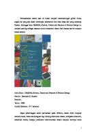
Color Theory and Its Application in Art and Design Second Completely Revised and Updated Edition



With 139 Figures and 23 Color Plates



Springer-Verlag Berlin Heidelberg GmbH



GEORGE A. AGOSTON



4 Rue Rambuteau, F-75003 Paris, France



Editorial Board



Professor KmcHI SHIMODA Faculty of Science and Technology Keio University, 3-14-1 Hiyoshi, Kohoku-ku Yokohama 223, Japan



DAVID L. MAcADAM, Ph. D. 68 Hammond Street Rochester, NY 14615, USA ARTHUR



L.



SCHAWLOW,



Ph. D.



Department of Physics, Stanford University Stanford, CA 94305, USA



Professor ANTHONY E.



SIEGMAN



Electrica! Engineering E. L. Gintzton Laboratory, Stanford University Stanford, CA 94305, USA THEODOR TAMIR,



Ph. D.



Polytechnic University 333 Jay Street Brooklyn, NY 11201, USA



ISBN 978-3-540-17095-2 ISBN 978-3-540-34734-7 (eBook) DOI 10.1007/978-3-540-34734-7



Library of Congress Cataloging-in-Publication Data. Agoston, George A., 1920-. Color theory and its application in art and design. (Springer series in optica! sciences ; v. 19) Bibliography: p. Includes index. 1. Color. 1. Title. II. Series. QC495.A32 1987 535.6 86-29685 This work is subject to copyright. Ali rights are reserved, whether the whole or part of the material is concerned, specifically the rights of translation, reprinting, reuse of illustrations, recitation, broadcasting, reproduction on microfilms or in other ways, and storage in data banks. Duplication of this publication or parts thereof is only permitted under the provisions of the German Copyright Law of September 9, 1965, in its version of June 24, 1985, and a copyright fee must always be paid. Violations fali under the prosecution act of the German Copyright Law. © Springer-Verlag Berlin Heidelberg 1979 and 1987



Originally published by Springer-Verlag Berlin Heidelberg New York in 1987 The use of registered names, trademarks, etc. in this publication does not imply, even in the absence of a specific statement, that such names are exempt from the relevant protective laws and regulations and therefore free for general use.



Foreword



This book directly addresses a long-felt, unsatisfied need of modern color science - an appreciative and technically sound presentation of the principles and main offerings of colorimetry to artists and designers, written by one of them. With his unique blend of training and experience in engineering, with his lifelong interest and, latterly, career in art and art education, Dr. Agoston is unusually well prepared to convey the message of color science to art and design. His book fulfills the hopes I had when I first heard about him and his book. I foresee important and long-lasting impacts of this book, analogous to those of the epoch-making writings by earlier artist-scientists, such as Leonardo, Chevreul, Munsell, and Pope. Nearly all persons who have contributed to color science, recently as well as formerly, were attracted to the study of color by color in art. Use of objective or scientific methods did not result from any cold, detached attitude, but from the inherent difficulties of the problems concerning color and its use, by which they were intrigued. Modern education and experience has taught many people how to tackle difficult problems by use of scientific methods. Therefore - color science. Few artists or others who deal with color will deny that color poses difficult problems. Capable people, all well-disposed to art and the aesthetic approach, have recently added significantly to the knowledge of color and to ways of working with it. They always intended that their findings would be useful to artists and designers. Unfortunately, they have not succeeded in conveying that message, or their contributions, to those intended beneficiaries. This book by Dr. Agoston will, I think, be the bridge of color between the cultures of science and art, of which modern color scientists have dreamed but never succeeded in building. The book is understandable by all persons, no matter what their education or experience. Everyone is interested in color. This book has a lot for everyone, no matter how little they have to do with color, nor how little their acquaintance with or interest in mathematics or physics. No equations are used. There are many graphs. They can be understood by anyone who reads newspapers or news magazines. Each graph, and its meaning for color, is explained in simple words. Yet the book is not condescending or trivial.



v



Knowledgeable scientists will find facts and perspectives that are not found elsewhere, some of which will be new and stimulating, even to color scientists. Rochester, September 1979



VI



David L. MacAdam



Preface to the Second Edition



This new edition includes some updating, the expansion of the discussions of some topics, and the addition of new topics and illustrations. My aim is unchanged. I wish to make selected pertinent knowledge in color science accessible to artists and designers. I continue to adhere to the policy of avoiding the inclusion of mathematical equations and texts for which a technical background of the reader must be assumed. But, for the benefit of those who do possess a technical background, I have introduced a Notes Section (Appendix) in which some equations and supporting technical information are presented. The material in the Notes Section is supplementary; it is not required reading for a full comprehension of the main text. Chapter 11, entitled "Conditions of Viewing and the Colors Seen", is the major addition to the book. Here several selected topics in psychology and physiology are discussed that extend the scope of the preceding chapters. The topics are clearly within the domain of interest in art and design. They include: color response in vision, adaptation, afterimages, simultaneous contrast, colored shadows, edge contrast, and assimilation. The discussion of the physiology of the eye in Chap. 2 has been expanded somewhat in preparation for the material in Chap. II. Much of the discussion of afterimages in Chap. 11 deals with afterimage complementary pairs. This is the type of complementary colors considered by Goethe in his color studies and frequently employed by artists in the past. There are many discussions of afterimages in the old scientific color literature. The more recent study by M.H. Wilson and R.W. Brocklebank (1955) stands out as one that offers potentially useful information on complementary pairs. The discussion of the Goethe color circle in the first edition has been modified here to take afterimage complementary pairs into account. The discovery of the attribute brilliance by the color scientist R.M. Evans, referred to in Chap.3 of the first edition, does not seem to have stirred up much interest among those currently engaged in color vision research. Yet, in my view, it is a potentially useful concept for artists and designers. More recently, R.W.G. Hunt has considered in detail the attributes of perceived color and, in particular, their definitions. Both what he calls colorfulness and the brilliance identified by Evans are treated in this edition. Artists and designers are becoming increasingly knowledgeable about the utility of the CIE chromaticity diagram. The CIE 1931 chromaticity VII



diagram is the dominant tool employed in color specification today. However, increasing use is being made of the CIE 1976 chromaticity diagram, which is an approximately uniform version. A discussion has been introduced in which the latter is presented. The text concerning the especially important OSA Uniform Color Scales has been expanded and now occupies a chapter by itself (Chap.9). Diagrams are provided to identify both uniform color scales and uniform twodimensional color arrays in the OSA scheme. The CIEL UV and CIELAB color spaces possess similar potential value in art and design. These are both discussed in greater detail (Chap. 8). A number of sections in Chaps. 7 and 8 have been expanded, and the following new topics have been introduced: iridescent colors (liquid crystals), metameric illumination, color rendering, the German Standard Color Chart, and two Japanese color sample sets (Chroma Cosmos 5000, Chromaton 707). The change in the Swedish NCS scheme of notation was not included in the earlier edition of this book; the revised notation is presented here. In the Introduction of the earlier edition, I cited names of contemporary color scientists who have made technical contributions in areas that are particularly pertinent in art and design. Not surprisingly, I have since learned of other major contributors, and, if I attempted a new list, I fear that it, too, would be inadequate. Now I appreciate better the rather widespread concern in color science for the needs of artists.and designers. In the preparations for this new edition, I have had the help and support of a number of people. Once more I am particularly indebted to Dr. David L. MacAdam for his critical comments. I am thankful to him for providing the color photograph for Plate XII and the color samples used in preparing Plate XIII. I am grateful to Prof. Leo M. Hurvich for his attention to my numerous inquiries concerning his research, and to Miss Dorothy Nickerson and Dr. Fred W. Billmeyer, Jr. for their assistance on various occasions. In this edition, I have made use of information that had been generously offered six years ago by Mr. Kenneth L. Kelly, of the National Bureau of Standards, Washington, D.C., some of which I was unable to include in the first edition. I wish to acknowledge with thanks the help of French artist Yves Charnay who supplied the two photographs of his painting in liquid crystals for use in Plate III; of Dr. Takashi Hosono, President of the Japan Color Institute, Tokyo, who provided information about Chroma Cosmos 5000 and Chromaton 707, and supplied the photograph for Plate XI and the diagram for Fig.8.26; of Mr. Rolf G. Kuehni, Mobay Chemical Corp., Rock Hill, South Carolina, who provided the spectral reflectance curve for Fig. 7.19; and of Munsell Color, Baltimore, who provided photographs for Fig. 8.11 and Plate VIII and a set of CIEJMunsell conversion charts, which were used for the preparation of Figs. 12.1-9. I wish to thank, too, Dr. Nahum Joel for continued helpful discussions in the domain of physics. Again, the VIII



Documentation Services of the Eastman Kodak Co. at Vincennes, France, have aided by giving me access to their reference materials, and I am grateful for this help. These and others have contributed in various ways to my book. However, the decisions that I have had to make in writing the book are my own, and I accept the responsibility for what I have written. I appreciate, in particular, Marjorie's tolerance. When she married me, I was fully occupied as a painter. She certainly never dreamed that one day I would take on the demanding task of writing a book on color. Paris, March 1987



George A. Agoston



IX



Preface to the First Edition



My aim in this introductory text is to present a comprehensible discussion of certain technical topics and recent developments in color science that I believe are of real interest to artists and designers. I treat a number of applications of this knowledge, for example in the selection and use of colorants (pigments and dyes) and light. Early in the book I discuss what color is and what its characteristics are. This is followed by a chapter on pertinent aspects of light, light as the stimulus that causes the perception of color. Then the subject of the colors of opaque and transparent, nonfluorescent and fluorescent materials is taken up. There are sections on color matching, color mixture, and color primaries. Chapter 6 introduces the basic ideas that underlie the universal method (CIE) of color specification. Later chapters show how these ideas have been extended to serve other purposes such as systematic color naming, determining complementary colors, mixing colored lights, and demonstrating the limitations of color gamuts of colorants. The Munsell and the Ostwald color systems and the Natural Colour System (Sweden) are explained, and the new Uniform Color Scales (Optical Society of America) are described. Color specification itself is a broad topic. The information presented here is relevant in art and design, for those who work with pigments and dyes or with products that contain them, such as paints, printing inks, plastics, glasses, mosaic tesserae, etc., and for those who use colored lights, lasers, and phosphors. I believe that this book can be of use as an introductory text to others in art conservation and in industries and commerce concerned with printing, dyeing, plastics manufacture, etc., but I have not treated their particular technical problems and have not introduced their specialized terminologies. I have taken great care to present technical information in a simple yet undistorted manner. No background in science or mathematics is necessary to follow the text. Algebra is not employed, but graphs, which are indispensable in discussing the subjects, are used in an elementary way. I believe that readers who are familiar with graphical presentations of the sort found in daily newspapers and news magazines will have no difficulty in understanding the graphs in the book. ( ... ) The text is based on information drawn principally from the current technical literature in color science, a domain that is found by many to XI



be forbidding, especially because it extends into rather different scientific disciplines, principally psychology, physiology, and physics. Numbers within brackets, such as [2.4] and [8.26], indicate citations of books and articles listed in the References Section at the end of the book. The notation [5.6, 7] signifies Refs. 5.6 and 5.7. In some cases a further distinction is made by giving the page number of a book, as [Ref. 6.2, p.l71]. My interest in color is that of an artist. It had its start in my early teens when I began making oil paintings. Then there was a gap in my art career when I studied and worked twenty years as a chemical engineer. Later, when I returned actively to painting, I came under the influence of artist and teacher Richard Bowman, and my use of color in painting changed radically from realistic to fauve. The development of my interest in the technical aspects of artists' materials and in the subject of color relates somehow to my training and experience in engineering. However, I can point with certainty to my physicist friend Dr. Arthur Karp as the one who kindled my interest in the basic topic of color perception. I am indebted to Dr. David L. MacAdam for his critical reading of the manuscript, to Dr. Nahum Joel for his helpful comments on the first half of the text, and to Mr. Kenneth L. Kelly for his suggestions concerning sections of the text dealing with certain work done at the National Bureau of Standards, Washington, D.C. I am thankful to personnel of the Documentation Services of the Eastman Kodak Company at Vincennes, France, for making reference materials available to me. Paris, September 1979



XII



George A. Agoston



Contents



1. Introduction ........................................... 1.1 Color Science and Art Before 1920 ...................... 1.2 Some Developments in Color Science Pertinent to Art and Design Since 1920 ................................



2



2. The Concept of Color ........•......................... 2.1 What Is Color? One Answer ........................... 2.2 The Visual System: A Brief Sketch ..................... 2.3 What Is Color? Some Other Answers ...................



5 5 6 8



2.4



1 1



What Is Color'? A Practical Answer in Technology ........



9



3. Perceived Colors ....................................... 3.1 Isolated Colors ....................................... 3.2 Hue ................................................ 3.3 Saturation and Colorfulness ........................... 3.4 Brightness and Lightness .............................. 3.5 Brilliance: Grayness and Fluorence ..................... 3.6 Color Terms .........................................



11 11 12 13 14 14 16



4. Light and Color ........................................ 4.1 What Is Light? ....................................... 4.2 Wavelength and Light ................................. 4.3 Spectral and Nonspectral Hues ......................... 4.4 Light from Lasers .................................... 4.5 Light from the Sun and from Lamps .................... 4.6 Standard Illuminants (CIE) ............................ 4.7 Eye Brightness Sensitivity .............................



17 17 18 19 21 21 24 26



5. Colored Materials ...................................... 5.1 Pigments and Dyes ................................... 5.2 Opaque Materials .................................... 5.3 Transparent Materials ................................ 5.4 Fluorescent Materials ................................. 5.5 Metamerism and Matching Colors ...................... 5.6 Additive Color Mixture ...............................



28 28 29 35 37 40 41 XIII



Subtractive Color Mixture ............................. Color Mixture by Averaging ........................... The Primaries ....................................... Color Circles .........................................



42 43 44 45



6. Color Specification (CIE) .............................. 6.1 Light and Color: Other Definitions ..................... 6.2 The Chromaticity Diagram: An Introduction ............. 6.3 The CIE Chromaticity Diagram ........................ 6.4 Dominant Wavelength and Purity ...................... 6.5 An Approximately Uniform CIE Chromaticity Diagram .,. 6.6 Metamerism and the CIE System .......................



47 47 48 53 58 62 65



7. Diverse Applications of the CIE Chromaticity Diagram 7.1 Color Names for Lights ............................... 7.2 Additive Complementary Color Pairs ................... 7.3 Colors Obtainable by Mixing Light ..................... 7.4 Light Called "White Light" ............................ 7.5 The Color Limits for Materials (Paints, Inks, Dyes, etc.) 7.6 Fluorescent Paints and Dyes ........................... 7.7 Iridescent Colors: Liquid Crystals ...................... 7.8 Mixing Paints ................... " . . . . . . . . . . . . . . . . . . . 7.9 Color Images in Television, Pointillism, Four-Color Printing, and Photography ..................................... 7.10 Color Difference ...................................... 7.11 Colors of High Contrast ............................... 7.12 Metamers ........................................... 7.13 Metameric Illumination ............................... 7.14 Color Rendering ...................................... 7.15 Color Temperature ...................................



66 66 68 70 72 74 79 80 83



5.7 5.8 5.9 5.10



8. Color Systems .......................................... 8.1 CIE Color Space, CIE(x, y, Y) ......................... 8.2 CIELUV and CIELAB Color Spaces .................... 8.3 Color-Sample Systems ................................ 8.4 The Munsell Color System. . . . . . . . . . . . . . . . . . . . . . . . . . . .. 8.5 The Color Harmony Manual and the Ostwald Color System. 8.6 The German Standard Color Chart ..................... 8.7 The Natural Colour System (NCS) and the Swedish Standards Color Atlas ................................ 8.8 Chroma Cosmos 5000 and Chromaton 707 ............... XIV



86 90 92 94 96 98 100



105 105 107 112 114 123 129 133 138



9. Color Systems (Continued): The OSA Uniform Color Scales ...................... 9.1 Equally Spaced Colors .............................. 9.2 OSA Color Space. . . . . . . . . . . . . . . . . . . . . . . . . . . . . . . . . . . 9.3 Uniform Color Arrays on the Series of Horizontal Planes Through OSA Color Space .......................... 9.4 Uniform Color Arrays on the Two Series of Parallel Vertical Planes Through OSA Color Space ............. 9.5 OSA Uniform Color Scales (OSA-UCS) ............... 9.6 Uniform Color Arrays on the Four Series of Parallel Oblique Planes Through OSA Color Space ............. 9.7 The Pastel Color Samples ........................... 9.8 Comments About the OSA Samples ..................



10. Color Names and Notations and Their Levels of Precision .......................................... 10.1 The ISCC-NBS Color Names of Materials .............



142 142 143 149 151 157 158 164 170



173 173



10.2 The ISCC-NBS Centroid Color Charts ................



178



10.3 The Dictionary of Color Names (ISCC-NBS) ........... 10.4 Color Designation: The Levels of Precision .............



178 179



11. Conditions of Viewing and the Colors Seen .......... 11.1 Psychological Aspects and Color Systems ............. 11.2 Hue Responses .................................... 11.3 A Psychological Color Specification System ........... 11.4 Adaptation to Color; Color Constancy ............... 11.5 Adaptation Level .................................. 11.6 Memory Color .................................... 11.7 Afterimage Complementary Color Pairs .............. 11.8 Simultaneous Contrast ............................. 11.9 Colored Shadows .................................. 11.10 Edge Contrast .................................... 11.11 Assimilation (Reversed Contrast) ....................



181 181 182 184 188 194 194 195 199 203 206 208



12. Appendix ............................................ 12.1 Some Useful Addresses in the Field of Color ..........



210 210 210 210 210 211



A) B) C) D)



Major Collections of Books on Color .............. Color Research ................................. Color Standards ................................ Associations ...................................



xv



12.2 Conversion Table and Charts. CIE(x, y, Y) Notation/ Munsell Notation. . . . . .. . . . . . . . . .. . . . . . . . . . . . . . .. . . 12.3 Procedure for Determining ISCC-NBS Color Names ... 12.4 Notes ............................................



212 229 239



Color Plates I-XXIII. . . . . . . . . . . . . . . . . . . . . . . . . . . . . . . . . . . . .



249



References ..............................................



269



Name and Subject Index ................................



279



XVI



1. Introduction



1.1 Color Science and Art Before 1920 Scientific aspects of the phenomenon of color perception have captured the interest of artists, musicians, and writers during the past two centuries. The German poet Goethe made many detailed observations about color perception and presented his ideas in a book entitled Farbenlehre (Theory of Colors) (1810) [1.1,2], which in the opinion of a prominent color authority Deane B. Judd (1900-1972) "may come to be recognized as foreshadowing, however dimly, the next important advance in the theory of color" [Ref. 1.1, p. xviJ. J.M.W. Turner studied Goethe's book on color and produced some compositions based on it [1.3]. His lecture notes at the Royal Academy reveal his interest as well in the work of the scientist-mathematician Isaac Newton on light and color [IAJ. In France, Eugene Delacroix applied principles that he had learned from De la loi du contraste simultane des couleurs (The Principles of Harmony and Contrast of Colors) (1839) by MichelEugene Chevreul, chemist and director of the dye houses of the Gobelin Tapestry Works outside (now inside) Paris [1.5,6]. Neo-impressionists Georges Seurat and Paul Signac were profoundly influenced by the book Modern Chromatics (1879) by the American artist-physicist Ogden Nicholas Rood and applied their knowledge in their divisionist paintings [1.5,7]. In recent years, new interest in Chevreul's book has been stimulated by the artist Josef Albers (1888-1976) at Yale University [1.8-10] and by the work of Op artists who have sought ways to heighten color brilliance. A.H. Munsell (1858-1918), artist and teacher at the Massachusetts Normal Art School (now the Massachusetts College of Art) (Boston), was particularly interested in finding an appropriate method for teaching color to children [1.11 J. He devised a practical color-notation system that had a scientific basis to serve as a teaching aid. Within several decades his system assumed great importance in color science and in color technology. In 1905 Munsell complained of "the incongruence and bizarre nature of our present color names" [1.12J. Pointing out that "music is equipped with a system by which it defines each sound in terms of its pitch, intensity, and duration," he reasoned that color should "be supplied with an appropriate system based



on the hue, value, and chroma of our sensations .... " The Munsell color system now serves as one important means for color specification. Other roles have been found for it. Munsell himself proposed how it could be used in choosing harmonious colors [Refs. 1.13, p.129; 1.14]. Color harmony has been discussed by Goethe [1.1], Chevreul [1.6], Rood [1.7], and the chemist Wilhelm Ostwald (1853-1932) [1.15-17]. The subject of color harmony has been treated in a book on colorimetry by Judd and Wyszecki [Ref. 1.18, p.390], more generally by Judd in a well-illustrated booklet [1.19]' and analytically by Burnham, Hanes and Bartleson [Ref. 1.20, p. 214].



1.2 Some Developments in Color Science Pertinent to Art and Design Since 1920 Denman Ross (1853-1935) and Arthur Pope (1880-1977) introduced color theory to their art and design students at Harvard University (Cambridge, Massachusetts) more than fifty years ago [1.21,22]. In that early period, Byron Culver (1894-1971) also presented the same subject at the Department of Applied Art of the Rochester Atheneum and Mechanics Institute (now the Rochester Institute of Technology) (Rochester, New York) [1.11]. Similar courses have been offered at many other art schools and departments of art and design of universities. But the examples set by Ross, Pope, Culver, and undoubtedly others were evidently exceptions. In 1942, R.B. Farnum of the Rhode Island School of Design reported, following a survey, that sometimes such subjects were treated only incidentally and that too little time was allotted to them. Some entrusted to teach color theory were incompetent or insufficiently interested [1.23]. Today, undoubtedly because of the impact of new developments in science and technology, more art schools and departments of art and design are giving fuller attention to the teaching of pertinent topics in the area of color science. Art teachers and artists are writing articles about their applications of color theory and their color research [1.24-31]. The international art journal Leonardo, which treats contemporary visual art, with full recognition given to pertinent aspects of science and technology, has presented a number of diverse articles on the subject of color. In commerce and industry, much attention has been given to color specification. For this purpose, Munsell implemented his color system with a large set of very carefully prepared color samples. The samples were related to one another through progressive changes of approximately equal steps of Hue, Value, and Chroma. For diverse applications, a number of other sample systems have been devised that are charcterized by other features. Common to most such standardized systems, each of which has hundreds of samples, is the practice of assigning numbers or codes to the colors. 2



Thus, colors matched to a standard sample are identified precisely by the corresponding number or code. This procedure is useful for communication, in commerce for example, where the use of color samples themselves would be inconvenient. An internationally accepted method developed by the Commission Intern at ion ale d'Eclairage (CIE) is widely employed for specifying color. It is based on the fact that the relative amounts of three standard primary colors required in a mixture to match a color can be used to identify and specify the color. The CIE method has been applied in subsidiary ways as well, some of which are of particular interest to artists and designers. These applications refer to the simple graphical presentation that serves the CIE method. The graphical presentation provides a basis for selecting, for example, the color names for lights. It enables the prediction of the colors obtainable when two or more lights of known color are mixed. In another application, the change of color quality (hue and purity) is traced when paints are mixed and when the color of a paint film fades with time. The graphical presentation also provides a basis for selecting additive complementary colors. Also, the upper purity limits for colors of nonfiuorescent pigments and dyes can be shown on the graph, for comparison with the purities obtained with presently available paints and inks. Furthermore, the CIE scheme is a stepping stone to other schemes that provide for precise determination of color differences. This is of particular interest to those concerned with close control of color differences in their work and to those wishing to know specifically about the precise degree of color change (as in a fading or deterioration of pigments). Both the Munsell and the Ostwald color systems have been known to artists and designers for a long time. An adaptation of the latter system is represented by a collection of samples in the Color Harmony Manual [1.32], a collection provided primarily for use in design. A more recently introduced sample collection, the Swedish SIS Colour Atlas NCS (Natural Colour System) (1979) [1.33J, will probably be of great importance to designers, artists, and architects. The NCS, like the Munsell color system [1.34 J, provides color samples selected by visual means. Of great significance is the fact that anyone with normal vision can apply the NCS method of color judgment without the use of samples and color-measuring instruments. In 1977 a collection of samples was made available by the Optical Society of America, which provides many series of colors of equal color difference [1.35J. The collection has been produced for applications in art and design as well as for study in color science. In Japan a number of collections of color samples have been produced. The most outstanding ones for use in design are Chroma Cosmos 5000 (1978) and Chromaton 707 (1982) [1.36,37J. In the English language, there is a profusion of names for colors in art, science, and commerce. Many names apply to more than one color, and many colors are labelled by more than one name. In an attempt to establish 3



some order, one major effort has been made by the U.S. National Bureau of Standards (NBS) and the Inter-Society Color Council (ISCC) to produce and identify a set of about 300 easily recognized and consistent color names and to provide a dictionary that relates over 7000 currently employed color terms to the set. Thus, for example, the term "Hooker's green", familiar to many artists, but not all, can with the aid of the dictionary be replaced by the more universally recognizable terms "strong yellowish green" or "dark yellowish green", depending on Munsell Value and Chroma. The ISCC-NBS color names have been adopted by Webster's Third New International Dictionary [1.38] and are in wide use in commerce. However, artists and designers, who were also expected by the originators of the color-name system to derive direct benefit from it, often seem to be unaware of it. The advances in color science mentioned in the preceding paragraphs concern the rather specialized domain of colorimetry. By comparison, the subject of color vision is vast. It embraces several conceptual levels [Ref. 1.39, p.3]: anatomical (the path from eye to brain), physiological (chemical and electrical mechanisms), physical (the passage of light from source to retina), psychological (the gross response of the visual system), and esthetic (pleasure, well-being). In spite of the enormous amount of research that has been reported, many basic underlying facts have yet to be revealed before a complete description or overall theory of color vision can be devised. Some scientific topics in the psychological domain that are of real in-



terest in art and design are chromatic adaptation, color constancy, afterimages, simultaneous contrast, and assimilation. Many artists are familiar with these either from their formal studies or from practice. These topics are of fundamental importance in color science and are being actively studied. They are discussed in this book along with pertinent topics in colorimetry, physics, and anatomy. The important domain denoted by the word "esthetic" involves both psychology and philosophy; it is not treated in this book. Nevertheless, scientists are interested in it, as is suggested by their writings on color harmony (above). The fact that there are aspects of color science that are of practical interest to artists and designers has been recognized by color experts for a long time. In recent decades, many have contributed to color science in areas that are particularly pertinent to art and design. Their work has already made an impact on art conservation as practiced in museum laboratories. It seems ironical that, although students and professional artists are rather well acquainted with earlier developments, such as the Munsell and the Ostwald color systems, many are unfamiliar with the comparatively recent strides in color science that are not only available to them but are also intended, in part, for their use. I hope that this book will help to arouse their interest in this new knowledge.



4



2. The Concept of Color



2.1 What Is Color? One Answer The color authority R.M. Evans (1905-1974) pointed out that the word color "as it is used in ordinary speech ... has many different meanings" [Ref. 2.1, p.173]. Even in the scientific domains of chemistry, physics, and psychology it has different specialized meanings. Let us consider first an everyday usage of the word color, a usage that implies the concept that color is a property of materials. Thus a ripe tomato has the property of being red; snow, of being white; Mary's scarf, of being blue; etc. We accept that the color of a material or object is its color perceived in daylight. We also speak of the color of light and commonly consider color to be a property of light. Thus when we look at a red traffic light, we suppose that light of a red color is radiating to our eyes. The red disk produced when such a beam of light strikes a white wall seems to confirm that the light has a red color. The concepts of color as a property of materials and of light serve numerous practical needs in daily life, the most important of which are those of survival [Ref. 1.39, p. 7]. The concepts serve well in a host of ways in commerce, art, science, and technology. For these reasons, it comes as a surprise to many people that these concepts are incorrect. Perceived color is incorrectly given as a property of materials and as a property of light. Newton, discussing the subject of light in his book Opticks (1704), stated correctly, "Indeed, rays, properly expressed, are not coloured" [Ref.I.1, p. vii]. Another example of an incorrect concept that serves us well in daily life is the idea that the sun rises and sets every day. Objective observations reveal, however, that the sun is not revolving about the earth, producing a sunrise and a sunset every 24 hours; instead, the spinning of the earth on its axis (one revolution every 24 hours) cuts off our view of the sun at the moment we call sunset and permits our view of it again at the moment we call sunrise. The concepts of color as a property of materials and of light and the concept that the sun rises and sets every day will continue to serve us in many important ways. We should, however, be prepared for the frequent



5



instances when the concepts of color as a property do not apply. Here is one example: The colors of two dIfferent fabrics match in one illumination but not in another. If color is a property, why does the color change and why does the match not remain? (We shall see later in this book that metamerism is involved.) Here is another example: Using one green paint, an artist makes a circular opaque disk (about 3 em in diameter) in the center of each of two sheets of paper (20 X 20cm); one sheet is colored dull red and the other neutral gray, but both the red and gray have the same Value (Sect. 8.4). The disks will not be perceived to have the same green hue. Why does the color of the disk change when the color of its background is changed? (The visual phenomenon occurring here is called simultaneous contrast.)



2.2 The Visual System: A Brief Sketch Colors may be perceived with the eyes closed, in dreams [Ref. 2.2, p.176], and also when physical pressure is applied to the eyeballs or when certain drugs have been taken [Refs.I.39, p.6; 2.3, p.14]. (Obviously, these are situations where color is not a property of materials or a property of light.) With the eyes open, under the usual conditions of seeing colors, light enters each eye and becomes absorbed in its interior; a succession of events follows that leads to the production of a signal or sensation in the brain. The sensation makes us aware of a color. After stating that light "rays ... are not coloured," Newton wrote, "There is nothing else in them but a certain power or disposition which so conditions them that they produce in us the sensation of this or that colour" [Ref.I.1, p. vii]. But the awareness of color does not tell us what color is. Before we continue with the question, What is color? (Sect. 2.3), however, it will be helpful to consider briefly certain information concerning the visual system. When we look at a luminous object, such as a piece of red-hot iron, a glowing incandescent-lamp filament, or the sun, our eyes react to light radiating directly from the object and we see it. On the other hand, a nonluminous object, such as a tree or a table, must be illuminated to be seen that is, if light (in sufficient amount and of adequate quality) falls upon the object, some of the light will be diffusely reflected (scattered) and our eyes will react to the reflected light [Ref. 2.1, p. 54]. Out of doors, non luminous objects may receive light in beams radiating directly from the sun, but in general they receive sunlight indirectly, scattered by clouds l , clear sky 1 and 1 Light from clouds is sunlight scattered by water droplets. Dust particles and molecules (of oxygen and nitrogen, principally) in the atmosphere also scatter sunlight. The scattering by gas molecules is wavelength dependent, producing the blue color of the sky



[2.4).



6



Optic



Fig.2.1. Sche matic diagram of t he horizontal cross section of th e right eye (top view)



Vitreous humor



Pupil -



Fixotlon



OXIS



Aqueous humor



Sclero (white of the eye)



surrounding non luminous objects (foliage, walls, etc .). Indoors, during the daytime, scattered light and sometimes sunbeams enter through windows. At night, nonluminous objects often receive directly radiated light and diffused light from lamps and, importantly for surfaces in shadow, scattered light from surrounding nonluminous objects (furniture, walls, etc.). Light reaching an eye enters it through a clear liquid (aqueous humor) and passes through the pupil and the crystalline lens. It then traverses a bulk of jellylike material (vitreous humor) and falls upon and is absorbed by the retina, a thin covering extending over the rear inner surface of the eye (Fig.2.1) [Refs. 1.18, p.6; 1.20, p . 44; 2.2, p. 7; 2.5, p. 16]. The retina consists of 10 layers identified as nerve cells, nerve connections, and membranes [Refs . 2.2, Fig.2 .3; 2.3, p.114; 2.6, Fig. 3]. The light must pass through at least five layers before it arrives at the lightsensitive photopigment-containing receptor cells, where light is absorbed. The absorption of light by a cell results in a reversible chemical change in the pigment. The chemical change initiates a transformation involving an electrical change that, in turn, somehow influences certain cells closer to the surface of the retina in which spike electrical discharges are produced. This excitation is transmitted through optic nerve fibers from each eye to the opposite half of the brain, to a part called the lateral geniculate nucleus (LGN), and from there on to visual centers at the rear of the brain. In the brain, sensations are produced that reveal aspects of appearance of the objects in view. Several such aspects are size, position, color, glossiness, texture, opacity, and transparency. The fact that there are some interconnections between juxtaposed nerve cells, which permit light that falls on one part of the retina to affect what is seen in another part, is cited as an explanation of visual phenomena such as simultaneous color contrast [2.6]. There are two types of light-sensitive receptor cells in the retina, known as rods and cones (because of their shapes) [Ref. 2.3, p . 116]. The rods, which respond only to light and dark, are characterized by high sensitivity; they 7



are capable of responding to light of very low intensity. The rods enable us to see in dimly lit rooms or in moonlight. At such low levels of illumination we are unable to distinguish hues (reds, yellows, greens, etc.) and we cannot discern detail as well as we can in daylight [Ref. 2.5, p. 17]. At very low light intensities the cones, which are responsible for color vision, are considered not sensitive enough to respond. Our vision at very low light intensities, essentially without color response, is called scoptic vision [Note2.1]. When the level of illumination is sufficiently high - that is, within the range of illuminance produced by street lighting and bright sunlight [Ref. 2.7, Fig.2] - the cone system responds. It is presumed that the rod system is then more or less saturated and hence incapable of producing significant variations in response [Ref. 2.8, p.569]. We then perceive colors and experience photopic vision. There are three classes of cones. In recent versions of the opponent-color theory of color vision, the three classes of cones are red-, green-, and blue-producing. It is assumed that, by appropriate interactions involving two or three classes, all the achromatic and chromatic colors, over the full range of brightness level (in photopic vision), can be produced (grays, red yellows, yellow reds, red blues, blue reds, green yellows, yellow greens, green blues, blue greens). When an eye is focused on an object, its image falls on (or across) a small depression in the retinal surface called the fovea (Fig.2.1). This region differs from the surrounding retinal area in that the layers through



which light must travel before reaching the receptor cells are thinner. The receptor cells in the central region of the fovea (subtending an angle of vision of 1°) are all cones (about 25000 of them!). The cones are more densely packed and longer than cones elsewhere. In the surrounding area of the fovea (subtending an angle of 2° or more), some rods are present, but they are relatively few at angles less than about 10°. Hence the fovea's center is the region of highest visual acuity in photopic vision [Ref. 2.2, p. 9]. The fovea determines the fixation axis when we focus our eyes on a detail (Fig. 2.1). There is a relatively small range of illuminance at which both rods and cones respond significantly and contribute to what is seen. Then "twilight vision" (mesopic vision) is experienced [Ref. 2.5, p. 18].



2.3 What Is Color? Some Other Answers Now let us return to the question, What is color? The psychologist L.M. Hurvich poses this question in his book [Ref. 2.3, p.13]. He asks whether an object has color because of its physical-chemical makeup or whether illumination constitutes the color of the object. Continuing, he asks whether color 8



is a photochemical event in the retina, a neural brain-excitation process, or a psychical event. His answer is, "Color is all these things ... ," but he adds that, before exploring these topics, "the main point to be made is that our perception of color ordinarily derives from an interaction between physical light rays and the visual system of the living organism. Both are involved in seeing objects and perceiving color." Kuehni devotes the first chapter of his book to the question, What is color?; in it he discusses physical, physiological, psychological, and psychophysical aspects. In answer to the question, he proposes a psychologically oriented definition: "Color ... is an experience, poetically speaking a flower of our brain activity" [Ref. 1.39, p. 7]. He deplores the official proposal of the following "circular" definition of color for scientific use. But I quote it here because it does convey a related psychological meaning: "Perceived color is the attribute of visual perception that can be described by color names: White, Gray, Black, Yellow, Orange, Brown, Red, Green, Blue, Purple, and so on or by combinations of such names." In his book on color, Evans introduced the question in a way similar to that of Kuehni. In much the same way as Hurvich, he wrote, "Any attempt to arrive at a definition of the word involves one at once in all the complexities of vision" [Ref. 2.1, p. 1]. In discussions of color perception, the term color stimulus (or simply stimulus) is generally used to refer to the light that arrives at the retina. Perception of a color by the brain is designated by the term color response (or simply response). The words "stimulus" and "response" are used later in this book where reference is made to color perception.



2.4 What Is Color? A Practical Answer in Technology Color scientists and technologists interested in quantitative means for specifying and measuring color have avoided the "complexities of vision" by defining color to be a characteristic of light, the stimulus. Indeed, color is a topic in the domain of psychophysics where a quantitative scheme has been devised - namely, the CIE-system, discussed in Chap. 6. To obtain an idea of the rationale of the psychophysical approach, let us consider the following hypothesis: Light enters the eye and is absorbed by the retina. A series of events is caused to occur that lead to the production of a signal or sensation in the brain. The sensation makes us aware of a characteristic of the light. Color is this characteristic. (Note that color is not a sensation.) Alternatively and equivalently, color is the characteristic of materials that results in their changing the characteristic of the illuminating light. Thus, the red color of a traffic light is a characteristic of the light; the 9



green color of a leaf is a characteristic of the leaf that produces a change in the characteristic of, say, the daylight in which it is found. (These same sensations, which are normally caused by light, can also lead to illusions of color when the eyes are closed, as in dreams or when pressure is applied to the eyeballs.) According to this hypothesis, the characteristic (color) of the light is its spectral power distribution (wavelength composition); the characteristic (color) of an opaque material is its spectral reflectance distribution, considered along with the characteristic (color) of the light illuminating the material (Sects. 4.5,6; 5.2). Thus, color, characterized in this way, is given by numerical data or curves representing the data. In science and technology, the color of light and of materials is commonly characterized by such curves. In addition, by means of a CIE method, such data can be combined with quantitative information that specifies the sensitivity of a typical human eye, to calculate a color designation (Chap. 6). The CIE numerical color designations are particularly useful because they can be identified with colors seen under standardized viewing conditions. The concepts of color as a characteristic of light and of materials bear a strong resemblance to the concepts of color as a property of materials and of light. These concepts refer to a stimulus. The difference is that, in the former concepts, color is a set of data and, in the latter, it is a subjective judgment of an aspe-::t of appearance.



10



3. Perceived Colors



3.1 Isolated Colors When we focus our eyes on a uniformly colored area of a painting, the color that we perceive is often influenced by the colors of surrounding areas. In the preceding chapter, it was mentioned that this psychological phenomenon is called simultaneous contrast. Artists and designers deal with it in striving for specific color effects. If, on the other hand, we wish to discuss or specify the precise color of a paint sample, for the sake of simplicity the sample should be considered in isolation, without the influence of colors of the surroundings, or in a standardized situation such as with a white or neutral gray background. When we see a red railway signal glowing from a distance at night in the absence of other lights, we are experiencing an isolated or unrelated color. The light received solely from one such source is called an isolated stimulus. Often the situation of an isolated stimulus is closely approached when the surroundings are not black if the intensity of the light (stimulus) greatly exceeds that of all of the surroundings. Usually it is not difficult to devise a way to receive light in isolation from a luminous object. But how can the light that is scattered from an object such as a piece of paper or a sample of paint be viewed in isolation? One way is to illuminate the object in an otherwise darkened room. Another way is to view the surface through an aperture or round hole in a black shield (reduction screen) while focusing on the perimeter of the hole. (The larger hole in the reduction screen inserted inside the back cover of this book may be used for this purpose.) The view of the uniformly colored surface some distance behind the screen should fill the hole. Because the black shield does not reflect much light, practically all the light received by the eye arrives through the hole from the surface of the viewed object. Also, because the hole's perimeter, not the object's surface, is in focus, the viewer gets the impression of a diffuse filmlike zone. (When the smaller hole is used, it should be held close to the eye.) Such color perceptions are not located in depth [3.1]; they are often called film colors or aperture colors. Aspects of the appearance of objects such as glossiness, transparency, and surface texture are eliminated when surfaces are viewed in this way. Or11



dinarily, these characteristics interfere with the assessment and comparison of surface colors [3.2]. For example, consider the task of selecting a silky fabric to match the color of a woolen fabric. Color that is perceived to belong to an object (self-luminous, like a lamp filament, or non-self-luminous like a dab of paint or a wine bottle) is called object color. The color of a non-self-luminous opaque object is often more specifically referred to as surface color. A film color is a nonobject color [3.1].



3.2 Hue Perceived colors have been found by Evans to have as many as five different attributes [Ref. 2.5, p. 94]. More recently, R.W.G. Hunt [3.3] and K. Richter [3.4] have called attention to the existence of several more. In the simplest case, that of isolated colors or film colors, there are just three attributes: hue, saturation, and brightness [Ref. 2.5, p.136J. Let us ask first: What is hue? When we look at a red light, we perceive a red hue. It is difficult to explain just what the perception of a red hue is, just as it is difficult to explain the perception of bitterness or the aural perception of shrillness. It is sufficient for our purposes to say that when we utter or write the word "red" , or the words "blue" or "purple" , we are conveying to others the idea of a particular hue. It has been estimated that a normal eye can distinguish about 200 hues [Refs. 2.1, p.ll8; 3.5J. Perceived colors that possess a hue are called chromatic colors; those that do not are called achromatic colors. We perceive an achromatic (hueless) color when we look at a glowing daylight fluorescent lamp, for example. We also perceive achromatic colors when we view white, neutral gray, or black surfaces illuminated by such a lamp or by daylight. It has been found that among all the hues there are only four that are not perceived as mixtures. These are called the unitary, or unique, hues [Ref. 2.5, p. 66J: unitary red, unitary yellow, unitary green, and unitary blue. All other hues are considered to be binary hues because they are seen as mixtures of the following pairs: unitary green and unitary yellow (yellowish greens and greenish yellows); unitary yellow and unitary red (reddish yellows and oranges); unitary red and unitary blue (magentas, purples, and violets); unitary blue and unitary green (greenish blues and bluish greens): It was mentioned in Sect.2.2 that three classes of cones have been identified in the retina. This is consistent with a hypothesis that states that three opponent pairs of psychological primaries (white and black, red and green, and yellow and blue) are involved in color vision [Refs. 2.3, p. 17; 2.5, p.107]. The four unitary hues are basic to this hypothesis. In Sect. 8.7 the 12



use of the four unitary hues and white and black in a practical method for judging colors is described, and in Sects. 11.2,3 their role in hue response and their application in a psychological color specification system are discussed.



3.3 Saturation and Colorfulness Perceived chromatic colors can generally be considered to possess a hue component and an achromatic component. Saturation is an attribute of perceived color according to which we judge the relative amount of the hue component in the color [Note3.1]. Let us consider two isolated beams of light, one red and the other pink. The beams are such that each evokes the same perception of hue and of brightness. The pink has the lower saturation because the relative amount (concentration) of the red component is less. L.M. Hurvich and D. Jameson have measured saturation coefficients quantitatively in their studies of color perception (Sect.11.3) [Refs. 2.3, p.79; 3.6,7). The saturation coefficient is calculated by dividing the amount of the hue component by the sum of the amounts of the hue and achromatic components. It is the fraction or percentage of hue in a color and is considered to be a quantitative measure of perceived saturation. There is no unanimity among color scientists on the precise definition of saturation [Refs. 1.39, p.39; 2.5, pp.1l9, 184; 3.3]. The above definition is ample for our purposes and is used in this book. Hunt has coined the term colorfulness for the attribute of perceived color according to which we judge the absolute amount of hue component in the color, irrespective of the amount of achromatic component present [3.3] [Note 3.2]. (Another term, chromatic ness, is also used to designate the same attribute [Ref. 1.39, pp. 39,48]). Thus, pink in the above example would be said to have less red hue than the color of the other beam. In other words, colorfulness applies to the absolute chromatic response experienced. Here is an example that demonstrates the difference between saturation and colorfulness. A piece of red paper illuminated by the beams from two identical spotlights in a darkened room has less colorfulness when one of the spotlights is turned off; less red hue is perceived. The saturation, however, is unchanged - that is, the concentration of red (the amount of red with respect to the total amount of red and achromatic content) does not change. Similarly, the color of a red dress viewed out of doors exhibits diminished colorfulness (but unchanged saturation) when viewed indoors under reduced illumination of the same quality. As Hunt has pointed out, saturation is the more important attribute of color for the recognition of objects. Colorfulness, on the other hand, depends on the illumination, a fact of real interest in art and design. 13



3.4 Brightness and Lightness Evans summarized in a book (1974) his thoughts and experimental evidence concerning the attributes of perceived color [2.5]. His discovery of the attribute brilliance may well be a major contribution to the science of color perception, but to accommodate brilliance among the other known attributes requires an expert reexamination of the respective roles played by each, particularly by saturation and by lightness. Brightness is an attribute of the illumination in which a nonisolated object is viewed [Ref.2.5, pp.96, 123]. Brightness commonly increases when the intensity of illumination increases. More precisely stated, brightness is the "perception of the general luminance level" [Ref. 2.5, p. 93]. (The term "luminance" is considered in Sects.6.2,3.) Brightness can refer to the perceived color of an object only when the object is isolated and light comes to the eye from the object and from nowhere else. For example, it is permissible to talk about the brightness of the color of light from a lamp or from a piece of paper illuminated by a spotlight observed in an otherwise darkened room. The visual experience of brightness is commonly described at the limits of its range as "dim" and "dazzling". Perceived lightness is an attribute of nonisolated colors (related colors). A related color would be perceived, for example, while viewing a green vase against a brown panel. Lightness is produced by the presence of a



second stimulus or of the surroundings [Ref. 2.5, pp.136, 137]. It commonly implies comparison, such as "lighter than" or "darker than" something else; it implies a perception of the luminance of light from one area relative to that from another or from the surroundings [Ref. 2.5, p.93]. We perceive lightness when we sense that more light is coming to our eyes from a piece of paper than from the brown table on which it lies. Evans has objected to the general practice of linking lightness to brightness in considerations of the colors of nonluminous objects. Thus, a definition beginning as follows would be considered misleading: "The term 'lightness' is used in place of 'brightness' to refer to surfaces ...." By such a definition, the perceptions of grayness and of darkness are incorrectly linked to brightness [Ref. 2.5, p. 93]. Evans' experimental work showed that brightness and lightness are separate variables, which had also been noted by others [3.3,3.8]. Furthermore, Evans placed the perception of grayness in a separate category, that of brilliance [Ref. 2.5, p.100].



3.5 Brilliance: Grayness and Fluorence Brilliance, like the attribute lightness, can be perceived only when the object viewed is not isolated, for example, an area of paint in a painting or 14



a piece of glass among others in a stained glass window. The perception of brilliance embraces two mutually exclusive aspects: either grayness is perceived or what Evans called fluorence [Refs. 2.5, p.99; 3.9], which is an apparent fluorescence or negative grayness [3.10]. To understand what is implied, let us consider a sheet of paper of a red color that possesses appreciable grayness when it is viewed in a room with normal illumination. In such cases, the light from the surroundings is more intense than that coming from the red sheet to our eyes. If, by means of a spotlight, a continuously increasing amount of light is directed onto the paper while the illumination falling on the surrounding objects remains unchanged, then the grayness of the red paper will decrease progressively and finally reach zero. At this point, the luminance of the light from the paper is still appreciably less than that of the light from the surroundings. This zero point is the separation between the regimes of grayness and fluorence (negative grayness). Then, as the spotlight illumination of the red paper is further increased, fluorence increases from zero (at the zero point) and the red acquires a fluorescent appearance; it is fluorent [3.9]. The fluorence continues to increase, but it finally reaches a maximum and then diminishes to zero. The maximum is reached when the lightness of the paper matches that of its surround. Above that lightness, the red appearance of the paper resembles that of a light source [Ref. 2.5, p.101]. A striking way to experience the grayness aspect of brilliance is to note the grayness of a sheet of neutral gray paper in a well-illuminated room and then the absence of grayness when the lights are turned off and the paper alone is illuminated by a white spotlight. In the latter instance, the paper is viewed in isolation, and the color perceived is white. Similarly, a paper colored brown, which is dark yellow or orange with added grayness, appears yellow or orange when it is viewed in isolation. It is interesting to note the difference between saturation and brilliance. As mentioned earlier, saturation concerns the relative amount (concentration) of the hue component perceived in a color. Saturation may vary from zero to nearly 100 %. Brilliance, on the other hand, concerns the absolute amount of grayness or of negative grayness present, each of which depends on the surroundings. Evans' recent discovery of brilliance as an attribute of perceived color has thus far received little attention in the current color literature (see, however, [3.4]), yet this attribute should be recognized by artists, designers, and others concerned with the application of color. Evans has pointed to the fact that Pope, in his book The Language 0/ Drawing and Painting (1949) [1.22, 3.11], showed an awareness of the need for an attribute such as brilliance [Ref. 2.5, p. 236]. Evans wrote: "There is no question ... of the fundamental soundness of his ideas, nor of the fact that a complete rewriting of that portion of his book in terms of the four variables, hue, saturation, brilliance, and lightness as we have developed them, would remove most, if 15



not all, of the ambiguities he encountered. Carrying out such a work would be a remarkable contribution to the understanding of the arts ... " [Ref. 2.5, p.235]. According to Evans, when related (nonisolated) colors of nonluminous objects are perceived, only four color attributes are involved: hue, saturation, lightness, and brilliance [Ref. 2.5, p.137]. Brightness is assigned to the illumination. As we shall see (Chap. 8), the attributes of perceived colors are sometimes used in important color systems. W.D. Wright [3.12] and A.R. Robertson [3.13] have discussed these attributes as employed in such cases.



3.6 Color Terms In the science of color perception, the terms "color", "hue", "saturation", "brightness" , "lightness" , "brilliance" , "red" , "blue" , "achromatic" ,etc., apply to color response. Used in this sense, they are terms of psychology. In the preceding sections, the attributes of color have been described in this sense. In later chapters where color measurement and specification are described, the frame of reference is changed. Color is linked to light (the stimulus) rather than to perception (the response) because precise measurements can be made on light relatively easily. For this reason, a new definition of color has been adopted, psychophysical color, that is satisfyingly close to the layman's everyday usage of the term "color". There should be no confusion in this book because the contexts within which the terms are used should provide the necessary clues. Whenever there is a need for clarity or emphasis, however, use is made of the specific terms "psychophysical color" (Sect. 6.1) and "psychological color" [Ref. 3.14, p. 229]. Artists and art writers seem to employ the terms "saturation" and "chroma" interchangeably to denote the purity of a color. The word "Chroma" is from the Munsell color system (Sect. 8.4). It is interesting that Munsell Chroma is intended to be a correlate of perceived saturation, but Evans has shown that it correlates more closely with a combination of saturation and brilliance [Ref. 2.5, p.168]. In art, the terms "value" ("Value" is used in the Munsell color system) and "tone" are often employed to denote lightness [Ref. 3.15, p.257]. The term "vividness" applied in art to colors might aptly refer to preceived brilliance. This is also suggested by the word "bright" as in "bright red" [Ref. 2.5, p.196].



16



4. Light and Color



4.1 What Is Light? What is light? A brief answer is: Light is a form of energy. Examples of other forms of energy are kinetic energy, such as that transferred from the wind to the vanes of a windmill, and chemical energy, such as that stored in an automobile battery, available for conversion to electrical energy. Light is a form of radiant energy. More precisely, light is electromagnetic energy, a category of radiant energy that includes x-rays, radio waves, etc. In Table 4.1 the various types of radiant energy in the electromagnetic category are presented. The whole range is called the electromagnetic spectrum. The Table 4.1. The electromagnetic spectrum. The visible spectrum occupies a small part of the electromagnetic spectrum. Wavelength is given in kilometers [km]' meters [m], centimeters [em], millimeters [mm J, and nanometers [nm 1



Radio waves



-----10 km ------1 km, 1000 m AM Short waves ------------100 m --------------10 m TV FM ---------------1 m, 100 ---------------------10 Radar ----------------------1



em em em, 10 mm



Microwaves - -------1 000 000 nm, 0.1 em, 1 mm



----------100 000 Infrared radiation -----------10 000 ------------1 000 Visible radiation --------------100 Ultraviolet radiation ---------------10 X-rays



nm nm nm nm nm



---------------1 nm ----------------0.1 nm ---------------0.01 nm



Gamma rays



----------------0.001



nm



17



relatively small range within it that represents visible radiant energy, is called the visible spectrum. We commonly define light as visible radiant energy [Note 4.1]. The term visible radiant energy for light implies correctly that the visual system responds to it in the experience of seeing. We know that it does not respond to radio waves. Nor does it respond to infrared radiation, ultraviolet radiation!, x-rays, and gamma rays, but eyesight can be destroyed by them. Only light is the stimulus to vision. The portion of the sun's radiation that penetrates the earth's atmosphere consists principally of visible, infrared, and ultraviolet radiation. This "mixture" reaches the earth's surface not only directly as sunbeams but also indirectly by scattering from water droplets in clouds and from dust particles, and by scattering produced by molecules (mainly nitrogen and oxygen) in the atmosphere (Sect. 2.2). As a result, infrared, ultraviolet, and visible radiation in various proportions falls on the earth from blue, hazy, and overcast skies. The radiation emitted by the hot tungsten filament of a common light bulb (incandescent lamp) and by the phosphors of a fluorescent lamp contains not only visible and infrared radiation but also some ultraviolet radiation.



4.2 Wavelength and Light Physicists tell us that electromagnetic radiation possesses a wavelike character. Indeed, measures of waves, such as wavelength and wave frequency, are used in the measurement of electromagnetic radiation. Only wavelength is used in discussions in this book, because it is the measure most commonly found in the literature on color. The classifications in Table 4.1 have been made on the basis of wavelength. Those who are familiar with the operation of radios know that if the wavelength of radio waves is reported, it is given in meters and kilometers. In the case of light, for which wavelengths are very much shorter, the unit of length commonly used is the nanometer nm. One nanometer is equal to one millionth of a millimeter (a millimeter is one tenth of a centimeter) and to one billionth (USA) or one thousand millionth (UK) of a meter. Until recently, in the literature on color, the use of units called millimicrons and angstroms was common. One nanometer equals one millimicron; one nanometer equals ten angstroms. 1 A portion of the spectrum of ultraviolet radiation is sometimes called "black light" because it is invisible ("black") in a darkened room and yet it excites fluorescence in many materials, causing them to glow and be visible in the dark (Sect. 5.4). It also affects photographic film in the dark.



18



4.3 Spectral and Nonspectral Hues Visible radiation is commonly considered to be represented in the electromagnetic spectrum in the wavelength range between 380 and 780 nm (Tables 4.1,2). A significant question is: What is perceived when light of a single wavelength (say 500nm) is viewed? The answer is: Green. At 600nm, it is reddish orange; at 470nm, blue. Table 4.2 shows the hues perceived for radiation over the whole visible range. Actually the hues change gradually when the wavelength is increased continuously from 380 to 780 nm. Thus, the greenish blue at 486 nm is more greenish than the greenish blue at 483 nm. Light of a single wavelength is called monochromatic light. The colors of the spectrum produced by monochromatic light have maximum saturation. Some investigators in color science consider that these colors contain an achromatic component and hence that they do not possess 100 % saturation (Sect. 11.3) [4.2,3]. Evans, on the other hand, believed that



Table 4.2. The visible spectrum and the nonspectral range



Color names for lights*



Hue wavelength range [nm]



Hue Relative complemen- lumitary wave- nosity length (Sect. range* 4.7) [nm]



~l~sl! E.ulJ>l~ lb!:) JV.iol~tlt __ J~O ___ ~6~ __ O.O~~~



Spectra 1 colors (visible spectrum)



Nonspectral colors



!:ur.pljs.h l2.Ju~(2.Bl(lUu~ -Qolel)t_ -46~ - - - - - - - ~'~75 ~ll!!! ~Bl - _ ~ _______ -482 ___ - - - - 0:15 t,~Q] ~~e~l ~G g~ - - - - - - -487 - - - - - - - 0.18 - - . .9 - - \£ - - - - - - - -493 - - - - - - - 0 24 ~l\!]sJ) ..9r~n_(~GL - - ____ -498- _ - - - - - 0·29 (ir§..ell.. (~L - - - - - - - - - -530 __ - - - - - 0·862 - - - - 1·00 y'el] ~'~hJl~e.!! LYCD - - ___ -558 y'eU~ ~r~en_(y'Gl - _____ -570:= := := __ - - 0·952 ren~Js~leUo~ i.gYj - - - - - -575 __ - - - - - 0:91 - - rt!.~ .L - - - - - - - - - -580 __ - - - - - 0 87 y'el]o~'2.h...9~n..9.eJy.QL - - - - -586 _ - - - - - - 0·80 Q.r~ng~ .lOL _________ -596 - - _ - - - - 0·68 ReQ.d~h_or..al!JleJ!:9L - - - - - -620 - - - - - - - 0·381 Red . ReQ. bR~ R____________ 6~0 ____ !~~~--0.17 !:.Ul.::P!..iS.hl~d_(e.Rl_ - - - - - ____ ~~e...ur.E El.{BP1_ - - - - - - ___ Re9..di~hYY.!'pJe_(d'L ________ Eur:plg IPl - - - - - - - - - - - - Bluish purple (bP)



--498c --528c _ -553c - -563c



t* Names for colored lights proposed by Kelly [4.1]. Names employed by other authors [4.1]. * Complementary wavelength with respect to CIE ILL C. (Sect. 6.4)



19



the colors produced by monochromatic light do not contain an achromatic component, with the possible exception of yellow [Ref. 2.5, pp. 73, 121]. Most light that we experience is not monochromatic. For example, a beam of blue light from a colored lamp may be found to contain light of wavelengths ranging over half of the visible spectrum. The major difference between a green beam and a blue beam from ordinary colored lamps is in the relative amounts of light contained in the green and blue wavelength regions. For example, a green beam has typically relatively larger amounts of light in the green region, from 500 to 550 nm, and a blue beam has larger amounts in the blue region, from 400 to 500 nm. The particular hue that is perceived is due partly to the predominance of energy in a wavelength region and partly to the brightness sensitivity of the eye (Sect. 4.7). Much of the light present at other wavelengths can be considered to "cancel out" chromatically by the mixture of additive complementary wavelengths (Sect. 7.2) producing an achromatic component that dilutes the dominant hue and hence lowers the saturation. When a beam of light from a lamp or from the sun is passed into an optical device called a monochromator, portions of the radiation can be isolated in wavelength intervals or bands, for example, in lO-nm wavelength intervals. Thus, a wavelength interval of light of SOO-SlOnm can be separated and projected onto a screen. In a device called a spectroradiometer [Refs. 1.20, p. 148; 2.1, p.ll; 4.4, p.29], each wavelength interval of light



over the visible range from 380 to 780 nm is separated and the rate at which radiant energy is received (power) within each interval is measured. A graph of power versus wavelength for the green and blue lamps discussed above provides a comparison of their wavelength compositions. Usually, however, the power data are converted to relative values to facilitate comparisons of their chromatic qualities, especially when the magnitudes of the powers of the light sources are appreciably different, e.g., a 25-watt (W) lamp, a 1000 W lamp, sunlight, etc. (Sect. 4.5). The hues represented by monochromatic radiation frqm 380 to 780 nm are those that are present in the sun's visible spectrum, a common example of which is provided by a rainbow. Those hues are called the spectral hues; all colors, regardless of saturation (the colors in a rainbow have low saturation), that are perceived to have a spectral hue are called spectral colors. But spectral hues are not the only ones that we commonly experience. There are also purple, purplish red, and a range of neighboring red hues that are not present in the sun's spectrum or in the spectrum of any source. Such hues are called nonspectral hues; colors having these hues are called nonspectral colors. Monochromatic radiation cannot produce nonspectral colors, but mixtures of two or more beams of monochromatic radiation of different wavelength can. Nonspectral colors of maximum saturation can be produced by combinations of, for example, monochromatic light of wavelength 680nm (red) and monochromatic light of wavelength 420nm (bluish 20



purple). Nonspectral colors of lower saturation are produced by beams that commonly contain light from most of the spectral range but with predominant amounts from the red and blue regions. A comprehension of the wavelength composition of light is aided very much by graphical presentations, which are discussed in Sect.4.5.



4.4 Light from Lasers Relatively recently, light sources called lasers have become commercially available. They can be used to produce monochromatic light. Because their light beams (called laser beams) commonly have radiation densities that greatly exceed those of light beams from ordinary lamps and of sunbeams, lasers are finding diverse uses in science, medicine, and technology. A laser beam consists of light in parallel rays and of one, two, or several wavelengths. The light is said to be coherent, which means that wave trains of energy are in step with each other, not out of step (out of phase) as in ordinary light [4.5]. Various media are used for the production of laser beams: crystals, glasses, gases (for example, argon, krypton, and mixtures of helium and neon), and solutions of dyes. Some gas lasers have been used as light sources in light art. Frequently, a helium-neon laser is employed, which produces a beam of monochromatic red light (632.8nm) [4.6,7]. Also, the use of an argon gas laser with a beam containing principally two wavelengths (488.0 nm, blue green, and 514.5 nm, green) has been reported [4.6]. In the latter case, light of the two wavelengths was separated by a diffraction grating to produce two monochromatic beams of different color [4.8]. Dye lasers can produce beams at any desired wavelength between 400 and 750nm [4.9-12]. At their present stage of development, dye lasers are exclusively pulsed devices; they require auxiliary equipment (an electronic flash tube or an additional laser) to drive them [4.13]. Of particular interest is the tunability of dye lasers, which permits the production of monochromatic light of any wavelength within ranges of 30 to 50 nm or more [4.11,12]. In the selection of lasers, very careful consideration must be given to their safety hazards. Outputs from lasers at power levels below 5 milliwatts (m W) have been employed in art displays, but even at such levels, certain precautions must be taken to ensure acceptable safety [Refs. 4.14, p. 7; 4.15, p.lOO].



4.5 Light from the Sun and from Lamps As mentioned in Sect. 4.3, most light that we experience is not monochromatic; an example of typical green and blue lights was cited. It is character21



istic of various light sources (the sun, a candle flame, a light bulb with an incandescent tungsten filament, a fluorescent lamp, etc.) that there are appreciable differences in the rates at which radiant energy is emitted (power) in wavelength intervals (say, of 10 nm) over the range from 380 to 780 nm. As noted before in Sect. 4.3, the wavelength composition of the radiation emitted by 'a source is most conveniently displayed by graphs showing relative power versus wavelength nm (Figs.4.1,2). Measurements of power are converted to relative power based in general on the convention that relative power has a fixed value of 100 at 560-nm wavelength. Thus, curves showing relative power for most light sources intersect at 560nm [Note4.2J. The wavelength-composition graph showing relative power plotted versus wavelength is called a relative spectral power distribution curve. (In earlier publications on illumination and color, the term "relative energy" was used; it has been replaced by "relative power".) Typical curves for light from an incandescent-tungsten-filament lamp and from a fluorescent lamp are shown in Figs.4.1,2. Comparison of the two curves reveals the relatively greater amount of radiation at 450 nm for the fluorescent lamp and at 650 nm for the incandescent light bulb. From the shapes of the two curves near 380 nm, it is clear that both extend to wavelengths below 380 nm and,



200



200



ISO



150



L.



Q.o



~a. Q.o



>



100



:.aa;



a:



50



o



400



600 500 Wavelength Inml



700



Fig. 4.1. Wavelength composition of light from a tungsten-filament lamp [typified by CIE ILL A (Sect. 4.6)]. Relative spectral power distribution curve. Color temperature: 2856 K



22



o 400



500 Wavelength



600



Inml



700



Fig.4.2. Wavelength composition of light from a daylight fluorescent lamp. Typical relative spectral power distribution curve. Correlated color temperature: 6000 K. (Based on data of Jerome reported in [Ref. 3.14, p.37])



hence, that the radiation from such fluorescent and incandescent lamps includes ultraviolet radiation. The relative spectral power distribution curve for the daylight-fluorescent-lamp radiation shows four vertical bars (Fig. 4.2). Each represents a wavelength interval, 10 nm wide, within which there is a tall sharp peak or jump of radiation that is characteristic for mercury vapor, which is in the tube. (The peaks occur at wavelengths of approximately 405, 436, 546, and 578 nm [4.16].) The smooth, continuous portions of the curve represent the radiation contributed by the phosphors in the lamp. The jumps, four monochromatic emissions from the mercury, are superimposed on, or mixed with, the diffuse multicomponent contribution from the phosphors. A precise indication of the relative magnitudes of the actual peaks would serve no useful purpose in the discussion of color. It is sufficient that each bar shown represents accurately the power averaged over a 10-nm wavelength interval. Figure 4.3 shows typical relative spectral power distribution curves for direct sunlight (I) and for north-sky light received on a 45° plane (II) at Cleveland, Ohio [4.17]. These two curves may be compared with a standard curve CIE ILL D65 (Sect. 4.6), which represents a typical phase of daylight. North-sky light in the northern hemisphere is judged to be "cooler" than direct sunlight, because it contains a greater proportion of light at shorter wavelengths (blue) and a lower proportion of light at longer wavelengths (red). Also shown in Fig.4.3 is a horizontal dashed line (E) which has been added to represent an equal power distribution - that is, a distribution in which the relative power does not vary with wavelength. This distribution



150



~ 100



3



o a. QJ



>



~ 50



300



400



500



600



Wavelength InmJ



Fig.4.3. Wavelength composition of direct sunlight (I) and north-sky light (II). The curves for CIE ILL D65 (Sect. 4.6) and the equal power distribution (E) are shown for comparison. Relative spectral power distribution curves. (Curves I and II are based on observations in Cleveland, Ohio, reported in [4.17))



23



serves as an arbitrary definition of a white light for purposes discussed later (Sects. 6.3, 7.2). Generally it is of interest because it can be regarded as a kind of intermediate representation for white light between the extremes of daylight and ordinary incandescent-lamp illumination [Ref. 2.5, p. 52]. A hypothetical light source capable of producing an equal power distribution (equal-energy light) is usually called an equal-energy light source.



4.6 Standard Illuminants (CIE) Because the perceived colors of objects generally vary with the illumination in which they are viewed, we tend to prefer to make color comparisons in daylight. But in color specification and color measurement, the wavelength composition of daylight must be specified precisely. For this reason, it has been found practical to establish internationally acceptable standards in the form of arbitrary wavelength compositions that represent typical sunlight, daylight, and artificial illumination. These standards, called CIE flluminants, have been established by the Commission Internationale d'Eclairage (CIE). (In the 1930s and 1940s, it was common in the United States to refer to the Commission by its English name or initials, International Commission on Illumination, I.C.I., but they



are no longer used [Ref. 4.18, p.4].) It is to be emphasized that the standard illuminants are, in reality, tables of numbers that state fixed wavelength compositions. Light having some of these wavelength compositions is produced in color-measurement laboratories with the use of special lamps and filters. Figures 4.4,5 show plots that represent several important CIE 11luminants. One illuminant, called CIE Illuminant A, or simply CIEILL A, represents closely the wavelength composition of light from a 500-W tungstenfilament light bulb (2856 K, Table 7.6) [Ref. 3.14, p. 47]. The relative spectral power distribution curve for CIE ILL A is given in Figs.4.1,4. Another illuminant, CIE ILL E, typifies the wavelength composition of direct sunlight at noon. The illuminant CIE ILL C is particularly important, because its wavelength composition is a close approximation to that of average daylight [Ref. 4.4, p. 7]. Most color measurements from the 1930s to the 1960s were reported in terms of CIE ILL C; some useful tools for considering colors relate to this illuminant (Sects. 7.1,5; 8.4-6,8; 10.1). The wavelength compositions of sunlight and of daylight are represented by CIE ILL Band CIE ILL C rather well, but only in the range from 400 to 700 nm. For the color measurement of fluorescent materials, illuminants should be used whose relative spectral power distributions in the wavelength range from 300 to 400 nm also typify those of sunlight and daylight. A new series of standard illuminants was introduced more recently that 24



150r-------------------------~



I-



'0, >'c, and pe Pigment used in film



Abbreviation



x



y



Y



[%]



>'0, >'c [nm]



pe



Cadmium red Madder lake



CR ML



0.5375 0.3985



0.3402 0.2756



20.78 33.55



604.8 496.5c



67.3 32.9



Cadmium orange medium Cadmium yellow light Zinc yellow Yellow ochre



COM CYL ZY YO



0.5245 0.4500 0.4486 0.4303



0.4260 0.4819 0.4746 0.4045



42.18 76.66 82.57 41.15



586.9 575.3 575.8 581.9



86.9 81.9 79.7 55.9



Emerald green Terre verte Viridian



EG TV V



0.2446 0.3092 0.2167



0.4215 0.3510 0.3635



39.12 29.04 9.85



511.9 549.8 497.1



22.8 9.2 31.9



Cobalt blue Ultramarine blue (natural) French ultramarine blue (artificial) Manganese violet



CB UB FUB



0.1798 0.2126 0.1747



0.1641 0.2016 0.1151



16.81 18.64 7.84



474.6 474.4 467.8



65.5 49.2 75.1



MV



0.3073



0.2612



26.99



553.7c



21.6



30



[%]



100~-------------_,



100~---------------,



75



75



t:., 0



~.,



YO



u



c



u



B 50



c



B 50 al



u ~



Q;



&



a::



25



Fig. 5.1



25



014--~-~~-'---'-~-~



1.00



500



600



O~-~--~--r-~~-,_-~



700



400



100---------------



75



t:.,



;!



c



c



0



.,



u



~



700



600



100~-------------_,



75



B u



500



Fig. 5.2



/,,-



u



B u 50



50



~



Q;



Q;



a::



a::



I



--- "



25



I



/



I



/



MV/ / /



/



Fig. 5.3



04---.---.--,----.---.-~



1.00 Wavelength [nmJ



500



600



700



Wavelength [nmJ



Fig. 5.1. Pigments. Cadmium red, CR (1); madder lake, ML (II). Spectral reflectance curves for matt pigment films. The CIE color designations are given in Table 5.1. (Based on curves in [5.9,10]) Fig. 5.2. Pigments. Cadmium orange medium, COM; cadmium yellow light, CYL; zinc yellow, ZY; yellow ochre, YO. Spectral reflectance curves for matt pigment films. The CIE color designations are given in Table 5.1. (Based on curves in [5.9,10]) Fig. 5.3. Pigments. Emerald green, EG; terre verte, TV; viridian, V. Spectral reflectance curves for matt pigment films. The CIE color designations are given in Table 5.1. (Based on curves in [5.9,lO]) Fig. 5.4. Pigments. Cobalt blue, CB; ultramarine blue (natural), UBi French ultramarine blue (artificial), FUB; manganese violet, MV. Spectral reflectance curves for matt pigment films. The CIE color designations are given in Table 5.1. (Based on curves in [5.9,10])



Fig. 5.4



100,----------------------------,



100-----------------------------,



Wh



75



75



~



~



OJ



OJ



u



c Cl U



~



u



c



Bu 50



50



2



Q;



Q;



0::



0::



25



Fig. 5.5 0 400



25



Wh/10Bk



Fig. 5.6



Bk 500



600



0 400



700



100



100



75



75



500



600



700



.



~



!:



OJ



OJ



U



c



u



c



B u 50



50 B u



OJ



't



~



&



0::



25



25



QR



Fig. 5.7 01+----,-----,...._--.-----,---,.-400



500



600



Wavelength Inml



700



Fig. O+_--,-_I~O~R~-_.--_,,...._-.---~ 5.8 400



500 600 Wavelength I nml



700



Fig. 5.5. Pigments and pigment mixtures. Carbon black, Bk; titanium dioxide white, Wh; mixture WhjOlBk (99%Whjl%Bk); mixture WhjlOBk (90%WhjlO%Bk). Spectral reflectance curves for glossy paint films (OSA-UCS) (Chap. 9). (Based on data in [5.11]) Fig.5.6. Pigments and pigment mixtures. Chrome yellow light, CYL; chrome yellow medium, CYM; indolinone yellow, IY; carbon black, Bk (Fig. 5.5); titanium dioxide white, Wh (Fig. 5.5); mixture CYLj30Wh (70 % CYLj30 % Wh); mixture CYLj80W (20 %CYLj 80 % Wh); mixture CYLjOlBk (99 % CYLjl % Bk). Spectral reflectance curves for glossy paint films (OSA-UCS) (Chap. 9). (Based on data in [5.11])



32



100',--------------------------,



75



..



o! u



c:



fl ~



I I



/-......



SO



I



I



Fig. 5.9. Pigments and pigment mixtures. Quinacridone magenta, QM; carbazole dioxazine violet, CDV; titanium dioxide white, Wh (Fig. 5.5); mixture QM/99Wh (1 % QM/99 % Wh); mixture CDV /99Wh (1 % CDV /99 % Wh). Spectral reflectance curves for glossy paint films (OSA-UCS) (Chap.9). (Based on data in [5.11])



1 ' 1 I \ I



'1;;



I



0:



,



\



I



\ CDV/99Wh \ \



"



25



I



.... ___ ..../'''......



/



/



'''''' QM



QM



o



CDV



400



soo



600



700



Wavelength (nml



For purposes of illustration, let us consider first the curve (I) for cadmium red in Fig. 5.1. It shows that the pigment exposed to daylight absorbs less than half of the light that it receives in the wavelength range above 600 nm and absorbs most of the light at wavelengths below 600 nm. Hence, mostly light of longer wavelengths (red) is scattered to the eye. Madder lake (II), however, absorbs smaller proportions of the light at wavelengths both above 600nm (red) and below 480nm (blue). The result is that when madder lake is illuminated by daylight a mixture of mostly long- and shortwavelength light (magenta) passes from the pigment particles to the eye. The spectral reflectance curves in Figs. 5.1-9 represent the simultaneous occurrence of diffuse surface reflection and selective absorption at wavelengths from 400 to 700 nm. Thus the scattered light that comes from selective absorption within the pigment particles is diluted at each wavelength by some surface-reflected daylight (typified for example by CIE ILL C). The spectral reflectance curve in the case of the cadmium red pigment (I) shows that below 550 nm about 5 % of the incident light was not absorbed. It



...



Fig. 5.7. Pigments and pigment mixtures. Phthalocyanine blue, PB; phthalocyanine green, PG; quinacridone red, QR; titanium dioxide white, Wh (Fig. 5.5); mixture PB/ 9S.SWh (1.2%PB/9S.S%Wh); mixture PG/90Wh (1O%PG/90%Wh); mixture QR/90Wh (10 % QR/90 % Wh). Over the range 400-700 nm, the reflectances of PB and PG vary between 4.1 and 6.5 %. Spectral reflectance curves for glossy paint films (OSAUCS) (Chap. 9). (Based on data in [5.11]) Fig.S.S. Pigments and pigment mixtures. Iron oxide yellow, lOY; iron oxide red, lOR; titanium dioxide white, Wh (Fig. 5.5); mixture lOY /SOWh (20 % lOY/SO % Wh); mixture IOR/SOWh (20 % lOR/SO % Wh). Spectral reflectance curves for glossy paint films (OSAUCS) (Chap. 9). (Based on data in [5.11])



33



is possible that surface-reflected daylight accounted for most of the 5 %. Davidson states that his data for high-gloss samples may be converted to data in which surface reflection is excluded by subtracting about 4 % from the reflectance at each wavelength [5.11J. Glossy paint films and varnished oil paintings often have colors of greater saturation than those of matt films that contain the same pigment. The reason is that, in the former, the pigment particles at the paint film surface are covered by a smooth glossy layer of paint vehicle (for example, dried linseed oil) or of varnish resin. In a red glossy paint film, for example, some of the scattered red light is reflected from the smooth surface back into the pigment particles again (internal reflection) where it is subjected to further selective absorption. This red light, which results from two passages of the light through the film, is combined with the red light that is not internally reflected and with surface-reflected white light to produce a mixture of light whose color is more saturated than the color obtainable with the same pigment in a matt film [Ref. 2.1, p.283J. The saturation of the color can be increased by viewing the glossy film when it is illuminated by a direct beam of light, such as a sunbeam. Even better results can be obtained by illumination with a projector beam in a darkened room, to avoid illumination with diffuse ambient light, which could produce diffuse, desaturating reflection in all directions. With isolated direct lighting, the white light that is specularly reflected from the surface, as from a mirror, can easily be avoided by a viewer, so that only undiluted scattered red light reaches the eye [Ref. 2.1, p.282J. The spectral reflectance curves in Figs. 5.1-9 are not accurate indicators of the wavelength composition of the light that comes from illuminated cadmium red and madder lake pigments [Note5.1J. The wavelength composition of the light that leaves a pigment film depends not only on the



150



~ ~



100



o a.



. >



.~



-;;



'"



100



34



600 Wavelength Inml



500



700



Fig.S.10. Madder lake pigment. Wavelength composition of light reflected from a matt pigment film (madder lake pigment [5.9,10]) when illuminated by daylight (II-C), typified by CIE ILL C, and by incandescent-lamp light (II-A), typified by CIE ILL A. Relative spectral power distribution curves. See Fig. 5.1



absorption characteristics of the pigment and on the surface reflection but also on the wavelength composition of the incident light. The effect of the incident light on the wavelength composition of the light from a pigment film is demonstrated in Fig.5.lD. Curve II-C is the relative spectral power distribution curve for the light coming from a madder lake film when it is exposed to daylight (typified by CIE ILL C). Curve II-A is for light that comes from the same pigment film when it is illuminated by an incandescenttungsten-filament lamp (typified by CIE ILL A). The marked difference in the wavelength compositions of CIE ILL C and CIE ILL A can be seen in Fig.4.4. Because light from incandescent lamps has relatively high radiant power at longer wavelengths (reds) and relatively low radiant power at shorter wavelengths (blues) (such light is often said to be "warm"), the light scattered by the pigment is richer in longer wavelengths and poorer in shorter wavelengths. Thus, in incandescent-lamp illumination, the madder lake pigment appears red, not magenta, because, as curve II-A shows, the blue content of the scattered light is very low.



5.3 Transparent Materials The phenomena that occur when light falls on a transparent material, such as colored glass or plastic, are essentially the same as those that occur when light falls on an opaque paint film. Part of the light that passes through the transparent (nonfluorescent) material is absorbed and dissipated, unnoticed, as heat; the remainder that is not absorbed emerges from the opposite side as transmitted light. (I am not now taking into account the simultaneous occurrence of internal reflection.) When daylight enters one side of a colored glass and red light is transmitted from the other side to our eyes, we say that the glass is red - that is, the perceived color (object color) is red. There is one difference to be noted, however. If an opaque matt red paint film is viewed in daylight, the red light that reaches our eyes from within the pigment particles is diluted by daylight that is reflected diffusely from the surface of the film. In the case of a transparent red glass, for example, there is also surface reflection of diffuse daylight, but this white light does not mix with the transmitted red light because it reflects from the glass in the opposite direction - that is, away from our eyes. A spectral transmittance curve for a red purple glass of 1-mm thickness is shown in Fig.5.11. The transmittance of a transparent material is the fraction or percentage of the incident light that passes completely through the material. A spectral transmittance curve is analogous to a spectral reflectance curve for an opaque material. The red purple glass allows red light (wavelengths longer than 630 nm) and blue light (wavelengths shorter than 480 nm) to pass through it; like the pigment madder lake, it absorbs most of the light of intermediate wavelengths. 35



100r--------------,



. . Fig. 5.11. Red purple glass. I-mm thickness. Spectral transmittance curve 1 0 0 r - - - - - - - - - -_ _~



75



., L



.,u



~



.,& 50



c



~ 50



,~



.,



.9



E VI c ~



'"



I-



•



25



200



SOO 600 Wavelength [nml



Wavelength



Fig.S.12. Red purple glass. Wavelength composition of light after it passes through I-mm (I) and 2-mm (II) thick glass. The light is from an incandescent lamp and is typified by CIE ILL A. Relative spectral power distribution curves



Figure 5.12 shows the relative spectral power distribution (curve I) for the light that emerges from the red purple glass of I-mm thickness when it is illuminated by an incandescent-tungsten-filament lamp (typified by CIEILLA) [Note5.I]. Because the relative amount of blue light (radiant power at lower wavelengths) in the lamp light is low (Fig.4.1), only a small amount of blue light is transmitted, as the small hump at the left end of curve I indicates. As a result, the color produced is reddish (pink) (chromaticity: 0.440, 0.279) (Fig. 7.1). [When daylight (CIE ILL C) passes through the glass, the color observed is purple (chromaticity: 0.261,0.144).] Curve II shows the relative spectral power distribution of the light that is transmitted in the case of two layers of glass or of one layer 2-mm thick. It is significant that the curves (Fig.5.12) move to lower positions when the number of layers or the layer thickness increases: the brightness of the transmitted light diminishes. It is also significant that the "valleys" decrease to lower positions faster than the "summits" (of the humps) [Note 5.2]; as a consequence the saturation increases and the hue may change. Now we might ask what occurs in the case of a transparent colored paint film on white paper. Let us consider the case of a paint film that has the characteristics shown in Fig.5.11. If light from an incandescent-tungstenfilament lamp falls on the paint film, curve I in Fig.5.12 could represent the wavelength composition of the pink light that reaches the surface of the paper after traversing the film. If we can assume that the white paper reflects all of the light that reaches it and that the reflection is diffuse, then the light will pass through the paint film again, but in the opposite direction, and will emerge as red purple light (chromaticity: 0.383, 0.168) having the 36



wavelength composition given by curve II (Fig.5.12) on reaching the film surface. The red purple light that emerges from the film surface will mix with the diffuse surface-reflected light (say 4 % of the incident light), and then, instead of curve II, another curve that includes the contribution of surface-reflected light will represent the total reflected light.



5.4 Fluorescent Materials Paints, inks, and plastics that contain fluorescent dyes are used commonly in advertising and decoration. The California artist Richard Bowman began using fluorescent lacquers in his paintings in 1950 [5.12]; the use of fluorescent paints and inks in art has been spreading widely. Many of the colors produced by fluorescent dyes viewed in, say, daylight cannot be produced by non fluorescent dyes and pigments under the same conditions (Sect. 7.6). In what way do the phenomena that occur in nonfluorescent and fluorescent materials differ when they are illuminated by daylight or lamplight? Here it is helpful to recall that, after light penetrates into an opaque or transparent nonfluorescent material, part of the received light is absorbed selectively and the remainder is scattered back or transmitted. The absorbed light is transformed to heat, which disappears unnoticed. It should be added that ultraviolet radiation that passes into a nonfluorescent material undergoes the same changes: part is absorbed selectively and transformed completely to heat, and the remainder is scattered back or transmitted as invisible radiation (ultraviolet). When visible radiant energy (light) and ultraviolet radiation penetrate into a fluorescent material, again some is scattered back or transmitted and the remainder is absorbed. What is different in the case of fluorescent materials is that only part (not all) of the absorbed light and ultraviolet radiation is transformed to heat. The remaining absorbed part is transformed and reemitted as visible radiant energy at longer wavelengths [Refs. 2.5, p.15; 5.13]. This transformed energy, reemitted as visible radiation, adds to the light normally scattered or transmitted from the material. The result is that, within certain wavelength regions, the light that leaves the surface is often increased sufficiently, in relation to the surrounds, to allow the visual perception of fluorescence. It should be pointed out that fluorescence can occur in some materials without evoking the visual perception of fluorescence [3.9]. Examples of fluorescent materials can be found in which only ultraviolet radiation is transformed to longer-wave visible radiant energy, but the materials of perhaps greater practical interest are those in which both ultraviolet radiation and short-wave visible radiant energy are transformed and produce what is called daylight fluorescence [5.14]. 37



An example of what may occur is indicated by the curves in Fig. 5.13 for a transparent fluorescent red film on paper exposed to sunlight [5.15]. Curve I shows the reflectance augmented by fluorescence contributions. At wavelengths shorter than 550 nm most of the light is absorbed. Within the wavelength range 580-680nm, the curve arches to 165 %, well above the horizontal dashed line that represents the spectral reflectance curve of an ideal white surface. It is clear that within an appreciable wavelength range more light is being emitted than is being received. The explanation is that part of the large amount of radiant energy (ultraviolet radiation and light) that is absorbed at wavelengths shorter than 580 nm is transformed and reemitted as light of longer wavelengths, from about 580 nm to over 700 nm. Curve II (dashed) is interesting because it shows results obtained when sunlight is filtered to eliminate all ultraviolet radiation (wavelengths shorter than 380 nm) before falling on the red film. The area between curves I and II represents the contribution (only about 10 %) made by the sun's ultraviolet radiation. Curve III indicates the portion that is not absorbed when the light received on the film is sunlight from which both ultraviolet radiation and light at wavelengths shorter than 580 nm have been filtered out to prevent fluorescence. Over the wavelength range 580-700nm, curve III is an ordinary spectral reflectance curve for the red film treated like a nonfluorescent material. The area between curves II and III is relatively great. It indicates



the significant contributions to wavelengths longer than 580 nm caused by transformation of radiant energy absorbed in the visible range between 380 and 580 nm. Knowing this, we should not be surprised to find that the red film appears red when it is illuminated with blue light [5.15]. Spectral reflectance and spectral transmittance curves for nonfluorescent materials are not dependent on the spectral power distributions of the light sources used for illumination. They are equally valid for incident light of all different wavelength compositions. The curves for fluorescent materials, however, do depend upon the wavelength composition of the illumination. Curve I in Fig.5.13, for example, is appropriate for the wavelength composition of sunlight in both the ultraviolet and visible domains at which absorption occurs. Figure 5.14 shows the reflectance curves appropriate for two different light sources, for the same colored sample. Curve I for sunlight (from Fig. 5.13) may be compared with curve IV, which is appropriate for illumination provided by an incandenscent-tungsten-filament lamp [Ref. 5.16, p. 36]. The lower peak is explained by the fact that less light and ultraviolet radiation are available at wavelengths shorter than 590 nm in a beam from the lamp (typified by CIE ILL A, Fig.4.4) than from sunlight (typified by CIEILLB, Fig.4.4). The difference of appearance with fluorescent and non fluorescent colorants is often so striking that we are tempted to ask what effects might be produced if they were mixed [Ref. 1.39, p. 111]. To understand the problem, 38



200,--------------__,



i.



~



150 -



1"



0;



~



-



g



100 ------------------- ---------



~



c



~ c



~



~



~



150



~g



-'! 100 ------------------------ --------



0::



200~-----------__,



~



0::



50



'00



500 Wavelength



700 Inm]



Fig. 5.13. Fluorescent red film on white paper. Spectral reflectance curves for illumination by sunlight (I), by sunlight with the ultraviolet portion filtered out (II), and by sunlight with all radiation below 580 nm filtered out (III). (From [Ref. 5.15, Fig.7J; reproduced with the permission of The Institute of Physics, Bristol, England)



50-



'00



500



600



700



Waveleng th Inm]



Fig. 5.14. Fluorescent red film on white paper. Spectral reflectance curves for illumination by sunlight (I) (from Fig. 5.13) and by light from an incandescent lamp (IV) (estimated on the basis of [Ref. 5.16, Fig. 9])



let us consider a mixture of cadmium red (Fig. 5.1) and the fluorescent red colorant (Fig.5.13) viewed in sunlight. From the above, we note that the fluorescent pigment absorbs radiation in the wavelength range 380-580 nm [radiation that is amply provided by sunlight (CIE ILL B, Fig. 4.4) land reemits a significant portion of the energy in the wavelength range 580700 nm in addition to the light scattered in that range. Cadmium red, on the other hand, absorbs about 95 % of incident radiation at wavelengths from 400 to 560 nm, which is dissipated invisibly (as heat). This means that most of the light of wavelengths below 560 nm that reaches cadmium red particles is lost and not available for scattering to neighboring fluorescent pigment particles (Sect. 5.7). Hence the fluorescent emission can be markedly reduced or eliminated, depending on the relative amounts of the pigments. If instead of cadmium red an equivalent amount of madder lake pigment (Fig.5.1) were used, the fluorescence would also be depressed, but perhaps not quite as much. The absorption of light by madder lake is less (say 65 % absorption) in the wavelength range from 400 to 560nm, as a result of which, more of the light scattered in this range by the madder lake particles would reach neighboring fluorescent particles. Optical bleaches (fluorescent brighteners) are used in paper and textile treatment. Such agents absorb ultraviolet radiation (in the wavelength range 300-400 nm) and emit part of it at short wavelengths in the visible range 39



(blue) (mainly 420-430nm) [Ref. 1.39, p.ll1]. The result is that yellowness in a fabric, for example, is "neutralized" (the blue emission adds to the scattered yellow light, its additive complementary color, to produce white light by additive color mixture, Sect. 5.6), and the lightness is enhanced by the increased amount of light that leaves the surface [5.15]. Some fluorescent pigments appear white or whitish in sunlight, but when viewed in darkness while exposed to "black light" (ultraviolet radiation, Sect. 4.1) they glow with highly saturated colors. Minerals that contain fluorescent constituents are often seen displayed in this manner in science museums. Their rich colors often cannot be seen in daylight, because their brightness is much too low in comparison with the brightness of ambient illumination.



5.5 Metamerism and Matching Colors Matching of colors involves a phenomenon that is fundamental to an understanding of the purpose and method of CIE color specification. It should be considered here, at least briefly. To introduce the idea, let us consider the following example. A small area of green paint has been scraped from a uniformly painted and uniformly illuminated wall. Now it is necessary to repaint the scraped area. House painters and willing artists are able to produce an excellent match even when the pigments in the paint they use are different from the pigments present in the surrounding old paint. But how can the match be a good one? Are not the spectral reflectance curves for the new and old paint films different? Yes, in answer to the second question, the spectral reflectance curves for the two paint films may be very different. The answer to the first question is related to the fact that the eye cannot identify the wavelength composition (relative spectral power distribution) of light [Ref. 2.5, p.25]. (In a way, the ear is more analytical than the eye, because it can detect each of the musical tones in a chord.) In fact, one color response, for example a particular green, can be evoked by anyone of a set of stimuli all of which have a different wavelength composition (relative spectral power distribution curve). This set of stimuli is called a metameric set. The stimuli in such a set are called metamers, and the matching property of such stimuli is called metamerism. In the case of matching paint, the stimuli (the light that comes to the eye from the two paint films) are matched. (The matched stimuli are metamers.) In reality, paints are not matched by the eye; only stimuli are. In addition, we should recall that the wavelength composition of the light that enters the eye depends not only on the spectral reflectance curves of the two green paint films but also on the wavelength composition of the light that falls on the paint films (Sect. 5.2, Fig. 5.10). If the wavelength composition of the illumination that falls on the "matching" paint films is 40



changed (for example, from that of light from an incandescent lamp to that of light from a fluorescent lamp), then it is almost certain that stimuli that come from the two films will no longer be metamers and that the perceived colors will be different; the "match" will no longer be good. The number of stimuli in a metameric set can vary widely. In the case of white light, the number of me tamers in the set is very large (Sect. 7.4). This means that light of a very large number of different wavelength compositions can produce the white response. The number in a set is much smaller when the colors of the spectrum are approached. Strictly speaking, for each of the colors of the spectrum there is just one stimulus - monochromatic light - in the metamer set. Thus the wavelength composition is given by one wavelength, for example, 495 nm for a certain bluish green spectral light. Judd estimated that there are more than 10 million metamer sets - that is, more than 10 million colors - that can be discriminated by comparison by an unaided normal eye under suitable viewing conditions [Ref. 2.5, p.29]. Light sources can be devised whose beams are metameric (metameric illumination [Ref. 2.5, p.217]). Startling demonstrations can be arranged with them. For example, a beam can be produced that is metameric with daylight, such that a sheet of paper (white in daylight) is also white in the beam, but a lemon (yellow in daylight) is reddish orange in the same beam (Sects. 7.4,7.13). A demonstration in color is given in [Ref. 2.1, p. 244, Plate XIII] showing the change of color of various objects under two metameric white illuminations.



5.6 Additive Color Mixture Just as the term "matching paint" is inaccurate, because in reality a stimulus light, not paint, is matched, so the term "color mixture" is inaccurate, because it is a stimulus light, not a response color, that is mixed. There would be some merit in replacing "color mixture" by a more scientifically correct term like "color-stimulus synthesis" [Ref. 1.20, p.1l5], just as there would be in replacing the usual commercial term "ice cream" by a term closer to the mark like "frozen milk product". But I am sure that it is more important both to be aware of the facts and to maintain general communication by using universally adopted terms. With this in mind, let us proceed to the subjects of additive color mixture, subtractive color mixture, and color mixture by averaging [5.17]. Additive color mixture occurs when light of different colors from two or more sources is combined (added together) before it reaches the eye. A helpful way to demonstrate the effect is to project two beams of colored light onto a white wall so that the two disks of light are superimposed and the combined light from the two beams is scattered from the wall. Because the two beams are added together, the energy in the combination is equal 41



to the sum of the energies of the two initial beams. Usually the effect is apparent in a resulting enhanced brightness when one disk is superimposed on the other (but there are exceptional situations [Ref. 5.18, p. 144]). If the perceived hues of the two initial beams are different, the resulting combined beam will generally be perceived to have an intermediate hue. Thus, if the beams are red and green, the hue of the superimposed disks may be yellow green, yellow, or orange, depending on the relative intensities of the initial beams. If, however, the hues are sufficiently different [at opposing positions on the color circle (Sect. 5.10)], for example a red and a blue green, then by appropriate adjustment of the relative light intensities it is possible to produce a hueless (white) response. In this case, the two original colors are called complementary colors [or, more precisely additive complementary colors (Sects. 6.2, 7.2)]. In general, the saturation of the color of the combined beam is less than that of at least one of the original beams. With complementary colors, of course, the saturation of the color of the combined beam can be as low as zero (white light).



5.1 Subtractive Color Mixture As described, additive color mixture can be demonstrated by the combination of two or more beams of light of different hues to produce a beam of yet another hue. Subtractive color mixture, on the other hand, can be performed with one beam, from which energy in different amounts at various wavelengths is removed (by absorption) by two or more different colorants such that the resultant beam produces a different hue. A beam of sunlight, for example, can be passed in succession through two pieces of colored glass (light filters), one yellow and the other green, to produce light of hue yellow green. When sunlight falls on the yellow glass, the yellow light transmitted has a wavelength composition that shows that most of the shorter-wavelength light (blue to green) is absorbed in the glass and that much of the intermediate-wavelength light (yellow green) and most of the longer-wavelength light (yellow, orange, and red) are transmitted. On the other hand, the green light produced when sunlight is passed through the green glass has a wavelength composition that shows that relatively large amounts of blue green, green, and yellow green light are transmitted and that most of the blue, yellow, orange, and red light is absorbed. From this, it is clear that when the beam of light is passed through one glass and then through the other, only the yellow green light emerges, because practically all light at other wavelengths is absorbed (subtracted out). Thus subtractive color mixture occurs when filters are "mixed" (placed in tandem) and light passes through them successively. The same process occurs, although probably not exclusively, when paints are mixed, for example yellow and green oil paints. A ray of light 42



that enters the paint film becomes scattered and passes in diverse directions through a mixture of yellow and green pigment particles, eventually emerging as yellow green light. Subtractive color mixture can also be demonstrated by passing a beam of light through a solution of two dyes. Again, each colorant (yellow or green dye) selectively absorbs light in its own way and the emerging beam is composed of wavelengths (yellow green) that largely escape both absorption processes. Because energy is removed from the beam by absorption, the intensities of the emerging wavelengths in subtractive mixture are always diminished. The effects can also be explained by using spectral transmittance curves for the green and yellow filters and by using spectral reflectance curves for the green and yellow pigments (Sects. 5.2,3) [Note5.1].



5.8 Color Mixture by Averaging Additive color mixture is the process of combining light beams of different colors before they reach the eye. However, beams can be combined in the visual process, as when light beams of different colors stimulate the same portion of the retina but without superposition. This can occur when the details in the retinal image produced by an array of tiny beams of different colors are more minute than is the "weave" or "mosaic" of receptor cells and interconnected nerve cells that respond to the array. In such a case, the different colors are not resolved and a kind of retinal mixture or blending takes place, which is sometimes called spatial averaging [Ref. 1.20, p.1l5]. A combination can also occur in the visual process when a rapid succession of flashes of light of alternating colors falls on an area of the retina. If the change is too rapid for the visual process to keep pace, retinal temporal mixture (temporal averaging) results [Ref. 1.18, p.66; 1.20, p.1l5]. In both cases, there is a "mixed" response: the mixed color is seen. These two kinds of combination (spatial and temporal mixture) are called color mixture by averaging. Thus, a printed paragraph of words in black letters on white paper becomes a gray area when viewed from a sufficient distance; the gray is the result of color mixture (black and white) by averaging (spatial mixture). The same occurs when juxtaposed dots of three different colors are viewed on a television screen, or in halftone printing on paper (Sect. 7.9). The same may occur when a pointillistic painting is viewed from so great a distance that the dabs of paint of different color are not individually distinguished. As the painting is approached and the individual color dabs begin to become distinguishable, other effects occur (Sect. 11.11) [Refs. 2.5, p.214; 2.6]. A good example of rapidly alternating stimuli leading to color mixture by averaging (temporal mixture) is a rapidly turning disk (sometimes called a Maxwell disk) whose surface has sectors of 43



different colors [Refs. 1.17, p.17; 1.18, p.66; 2.3, p.90J. Thus a disk whose surface is covered by black and white sectors will appear gray while turning. The difference between additive color mixture and color mixture by averaging is implied by the two terms. In additive color mixture, the energy of the two combined beams is the result of adding the energy of the two initial beams, and the brightness is usually (but not always) increased. In color mixture by averaging, the effective energies are area averaged or time averaged in the visual process, and a kind of average brightness is generally produced. The terms optical mixture and visual mixture are commonly used in reference to color mixture by averaging.



5.9 The Primaries To many people, the terms primaries and primary colors suggest bright red, yellow, and blue colors. With paints of these colors, and of white and black in addition, mixtures can be made that produce colors of a wide range of hues, lightness, and saturation. Because it is desirable here to consider color mixture and matching in a broader sense, the concept of the primaries as stimuli (light) will be further elucidated. A basic requirement of a set of three primaries is that no combination of any two of them matches the third [Refs. 1.20, p.119; 1.39, p. 73J. To have particular utility, the qualification is usually added that the three primaries be selected so that the gamut of colors obtainable by mixing them includes all hues and is as large as is practical. A very large gamut of colors (Hardy-Wurzburg gamut, Sect. 7.3) that includes all hues may be produced by mixtures (additive color mixture) of varying proportions of monochromatic light of three wavelengths: 700 nm (red), 535nm (yellowish green), and 400nm (bluish purple, or violet) [Ref. 2.1, p. 238J. The color gamut includes all the purples and most of the reds, oranges, and yellows; only the high-purity greens and blues are excluded (Sect. 7.3). Three such stimuli are called additive primaries. In a less specific way, the additive primaries are ordinarily said to be stimuli that produce the responses red, green, and blue. In some situations the subtractive primaries are of importance. The colors produced by each of the three subtractive primaries are complementary to red, green, and blue, - namely, cyan (blue green or turquoise), magenta (purplish red), and yellow, respectively. Cyan, magenta, and yellow pigments and dyes are used in color photography and in the four-color (including black, to improve blackness and definition) printing process. In these cases, there is an advantage in having to deal with only three or four dyes or inks. Admittedly, painters and designers, who use tubes or jars of paint of a great variety of colors, may not find the subject of subtractive pri44



maries directly relevant to their work, but, as will be shown in the following chapters, the additive primaries are basically relevant in art and design.



5.10 Color Circles Color circles of the type familiar to artists generally present color samples in the sequence of spectral hues, as found in a rainbow. A color circle is completed by inserting the nonspectral hues (purples and purplish reds) between violet and red. Colors can be selected to form a color circle such that pairs of complementary colors [additive complementary pairs (Sect. 7.2) or afterimage complementary pairs (Sect. 11. 7)] are directly opposite each other [Ref. 1.20, p.116]. A circle of six members may be formed that has samples that represent the three additive primary colors and their additive complementary colors, the subtractive primary colors (Fig.5.15 and Plate I). Intermediate complementary-color pairs may be introduced to increase the number of colors to 12, 24, 48, 96, or 192. But in a circle that contains 192 colors, the difference between the hues of adjacent colors is hardly perceptible (Sect. 3.2). F.J. Gerritsen, opposed to the old practice of teaching art students that the primary colors are blue, red, and yellow, has proposed a color circle of additive complementaries as a teaching aid [5.19,20J. Color circles containing 12 and 15 additive complementary pairs have served as the basis of several editions of an important color-sample atlas, the Color Harmony Manual [1.32] (Sect. 8.5). A six-member color circle consisting of three afterimage complementaryhue pairs is properly called a Goethe color circle, for Goethe is credited with



Fig.5.15. A six-member color circle. Opposing additive complementary pairs (Sect. 7.2)



Fig. 5.16. A Goethe color circle. Opposing afterimage complementary pairs (Sect. 11. 7)



45



its introduction [Refs. 1.2, pp.41, 49; 5.3, p.664J. Examples of such a circle are shown in Fig. 5.16 and Plate I. Goethe determined his "physiological complementaries" [Refs. 1.1, Sect. 3, p.2, Sect. 47, p.20; 5.21J, the term he used to refer to afterimage complementary pairs, in his studies of color contrast (1793). They were red/green, blue/orange, yellow/violet [Refs. 1.1, Plate I; 1.2, pp. 41, 49; 5.22, p. 205; 5.23J . If we wish to make a color circle of a relatively large number of colors (24,48, or 96, for example), we should consider the possibility of having an approximately visually uniform hue sequence with afterimage complementary pairs in diametrically opposing positions (Sect. 11.7). (An arrangement of equally spaced hues with additive complementary pairs in opposing positions has not been found [5.21J.) Furthermore, it should be noted that a circle based on afterimage complementary pairs has a more balanced appearance than one based on additive complementary pairs [Ref. 5.3, p. 664J. In the latter, there appear to be an excess of blue green hues and a deficiency in blue and red hues. Another type of color circle involves the four chromatic psychological primaries (unitary red, yellow, green, and blue) positioned at equal (90°) intervals (Sects.3.2, 8.7, 11.2). The binary intermediate hues yellow red (orange), red blue, blue green, and green yellow are located midway between the corresponding unitary hues. This type of circle is embodied in the Swedish Natural Colour System (NCS) described in Sect. 8.7 and in the Hurvich-Jameson HBS System (Sect. 11.3). NCS color chips and papers are available that may be used for the construction of circles containing 4, 8, 16, 32, ... members. Series of color samples whose hues differ by equal, or approximately equal, perceptual amounts are found in three well-established color-sample collections: The Munsell Book of Color (Sect. 8.4), The DIN-6164 Color Chart (Sect. 8.6), and the OSA Uniform Color Scales (Chap. 9). In making a color circle using color chips or papers from these collections, one can make selections taking full account of two other controlled variables. For example, in the Munsell collection one can select chips for a hue circle having a specific Value and Chroma (Sect. 8.4). A complete circle of approximately equally spaced Munsell hues would contain 40 chips.



46



6. Color Specification (CIE)



6.1 Light and Color: Other Definitions The subject of color measurement, colorimetry, is in the domain called psychophysics, which lies between the domains of psychology, physics, physiology, and chemistry [Ref. 4.18, p.40]. In the early 1930s, colorimetry was put on a universally accepted precise quantitative basis. The scheme, however, required a redefinition of basic terms. As stated in Sect. 4.1, we commonly define light as visible radiant energy [Note4.1]. In psychophysics, however, a definite distinction is made between light and visible radiant energy. Here the meaning of the term "visible radiant energy" is retained; it is radiant energy in the range from



380 to 780nm and the stimulus of vision [Ref.4.18, p.13]. Light, on the other hand, has been defined in psychophysics to take account of a human observer's awareness: light is "the aspect of radiant energy of which the human observer is aware through the agency of his eyes and the associated nervous system" [Ref. 4.18, p.40J. The distinction is clear if we consider that we are not equally aware of visible radiation received in equal amounts at 381 nm (barely visible) and 555 nm (of maximum visibility). Thus, in psychophysics "visible radiant energy" refers to all radiation in the visible range, and "light" refers to the same radiation but with the relative magnitude of its effectiveness in producing vision taken into account. With light considered in the psychophysical sense, we can proceed to the psychophysical definition of "color" , the "psychophysical color" mentioned in Sect. 3.6. The word "color" in psychophysics denotes a characteristic of the stimulus - that is, of the visible radiant energy. (This is closer to the layman's concept that light is colored). It takes into account both the radiant energy that reaches the eye and a standard observer who has typical normal color vision and, hence, makes typical use of the radiation that produces vision. The Committee on Colorimetry of the Optical Society of America, having adopted the psychophysical concept of color, reported, "This course seems to be amply justified on purely philosophical grounds, but, if less academic justification is desired, the purely practical considerations are fully sufficient" [Ref. 4.18, p.13]. Often, colors can be measured by finding a match to one of a series of standard samples (such as printed papers, dyed fabrics, and paint swatches or chips) under standardized conditions of viewing. For greater accuracy, 47



devices called colorimeters can be used. In one type of colorimeter, the field of view contains the color sample and the comparison color. The latter is varied by three kinds of adjustments until a match is found. The color is then expressed in terms of three numbers that, in the case of some instruments, represent directly the internationally accepted CIE tristimulus values (Sect. 6.3) or else can be converted to them. Photoelectric colorimeters operate automatically; in them the human eye is replaced by a photoelectric cell whose spectral responses are adjusted to mimic human vision. A colorimeter provides a direct measurement of color. There is, however, an indirect method that provides the CIE tristimulus values; it is more precise and quite extensively employed. The method involves the use of a spectrophotometer to obtain a spectral reflectance curve for an opaque sample (Sect. 5.2) or a. spectral transmittance curve for a transparent sample (Sect. 5.3). With use of the curve, the CIE tristimulus values can be calculated in a routine manner for the sample in a selected kind of illumination (for example, illumination typified by CIE ILL Cor CIE ILL D6s). The possibility of human error in making direct color measurements is avoided in this procedure. Imperfections of photoelectric-cell adjustment in colorimetry are also bypassed. This indirect approach is of particular interest because the scheme established for it provides access to the structure that underlies the CIE tristimulus values, which are basic to the precise specification of colors. Some of the fundamental ideas involved are taken up in Sects. 6.2, 3, and 5.



6.2 The Chromaticity Diagram: An Introduction Let us begin with the Maxwell triangle, the framework of the chromaticity diagram, which is in universal use in commerce, industry, and science and is now appearing in literature intended for artists and designers. The subject is easily approached by considering the example of three beams of light of short, medium, and long wavelengths used as a set of three additive primaries (blue, green, and red). Different colors are produced by superimposing the disks of the three beams projected on a white wall (additive color mixture) and varying the amount of light in each beam. If the color produced by a fourth beam of light is within the gamut of colors that can be produced by mixtures of the three beams, then the color can be specified by the amounts of each of the three beams (primaries) required to match it. A set of three additive primary colors and the complete gamut of colors obtainable by mixing two or three of them can be represented on a kind of mixture diagram, an equal-sided (equilateral) triangle, the so-called Maxwell triangle, named after the Scottish physicist James Clerk Maxwell (18311879), who employed it in his basic work on color. The three primaries are 48



Fig. 6.1. Chromaticity diagram or Maxwell tri-



angle (equal-sided triangle)



Magenta



assigned to points at the corners of the triangle. The gamut of colors of all possible mixtures of the particular primaries is represented by points on the three sides of the triangle and by points within it (Fig.6.1). The representation of psychophysical color by the triangle is partial. The part that is represented is called the chromaticity, and, indeed, it is now much more common to refer to the triangle as a chromaticity diagram. Chromaticity is the quality aspect of psychophysical color; it is a composite representation of approximate equivalents of psychological hue and saturation. The part not included on the diagram, the quantity aspect of psychophysical color, is the effective amount of light - that is, the amount of psychophysical light defined in the previous section. It is the amount sensed in the visual process. Because the eye's efficiency in responding to a given amount of radiation varies from zero at the limits of visibility (380 and 780nm) to a maximum at 555nm (Sect. 4.7), the psychophysical amount [called the luminance (Sect. 6.3)] is taken as the physical amount weighted by the eye's efficiency. A condition imposed on the selection of the colors to serve as primaries is that, when the three beams are combined in psychophysically equal amounts, a white disk is produced on a white screen or wall. The chromaticity of such an equal-energy white is represented by point E at the center of the chromaticity diagram (see also Sect. 6.3). Although the equal-sided triangular chromaticity diagram is employed rarely, it is instructive to consider it a bit further before we examine the diagram that is in present-day use. The equal-sided triangular diagram may be presented on triangular-coordinate paper, which is subdivided by three superimposed sets of parallel lines (Fig.6.1). The three sets are shown separately in relation to the triangle in Figs. 6.2-4. It is helpful to borrow the CIE symbols X, Y, and Z; these represent the CIE tristimulus values, which are defined for the particular set of primaries discussed in Sect. 6.3. Here, however, they are taken to represent the amounts of the three primaries now being discussed (X, amount of red; Y, 49



G



y =Q4



8



~------------------~y=O



R



Fig. 6.2. Lines of constant y (fractional amount of primary green) G



Fig.6.4. Lines of constant z (fractional amount of primary blue)



Fig.6.3. Lines of constant x (fractional amount of primary red) G



Fig. 6.5. Location of point S



amount of green; and Z, amount of blue) needed in a mixture to match a color within the gamut. The relative proportions or fractional amounts (given by x, red; y, green; and z, blue) clearly represent the quality aspect of psychophysical color and, as we shall see, they locate the chromaticity by a point on the chromaticity diagram. If the tristimulus values are X = 60, Y = 80, and Z = 60, then the fractional amount of primary red x, for example, is the amount of red (60) divided by the total amount (200), which is 0.3. The calculations similarly yield 0.4 for y and 0.3 for z [Note6.1J. The chromaticity of the color can now be represented on the diagram. Figure 6.2 shows a series of parallel lines along each of which y does not vary, for values of y from zero at the base of the triangle (0 % primary green in the mixture) to 1.0 at the vertex of the triangle (100 % primary green). Because y = 0.4, the sought point must be located somewhere on the line labelled y = 0.4, shown as a dashed line. Figure 6.3 presents similar information for the primary red. Because x = 0.3, the point must be 50



located on the line labelled x = 0.3. The point can be located on both lines simultaneously only at their intersection (Fig. 6.5). By use of Fig.6.5, the sought point S can be transferred to the chromaticity diagram (Fig. 6.1). It is clear that the information z = 0.3 and the point's location on a line labelled z = 0.3 in Fig.6.4 are not needed. Only two fractional amounts are necessary to locate the point and to specify the chromaticity; the two commonly employed are x and y. When values are given for x and y, the value for z can always be obtained by subtracting the sum of the values of x and y from 1.0. The chromaticity of the color just discussed is written as (x = 0.3, Y = 0.4) or, more commonly, as (0.3,0.4)' - that is, (x,y). In the case of white (equal-energy white), for which the amounts of the primaries required are equal, the fractional amounts x, y, and z are obviously each equal to 1/3, or 0.333, and the chromaticity is specified by (0.333,0.333). The central location of point E (Fig.6.1) can be checked by plotting the point by use of the procedure just described. Point Q that is plotted on one side of the diagram shows the chromaticity of a mixture of two primaries, red and green. For a mixture of equal amounts of primaries red and green (X and Yare equal, and Z is zero - there is no primary blue), fractional amounts x and yare equal, that is, 1/2, or 0.5 - and the chromaticity is (0.5,0.5). This chromaticity is represented by point J on the diagram and corresponds to yellow. Similarly, equal amounts of primary red and primary blue result (when the amount of primary green Y is zero) in a light beam that produces the color magenta (0.5,0.0) (point M); and equal amounts of primary blue and primary green result (when the amount of primary red X is zero) in the color cyan (0.0, 0.5) (point C). The sequence of the colors around the triangle (Fig.6.6) is the same as that in the six-member color circle showing additive complementary pairs (Fig.5.15). Additive complementary color pairs are found by drawing straight lines across the diagram, through point E, such as the dashed line that connects red and cyan (Fig.6.1). Constructing a line from point



Fig. 6.6. Superposition of the Maxwell triangle and a six-member color circle of additive complementary pairs. (From Fig.5.15)



51



Q (yellow green) through point E to the opposite side would show that the complementary color is a purple. More will be said about additive complementary colors in Sect. 7.2. The colors produced by mixtures of light are of maximum saturation when the chromaticities of the mixtures are located on the sides of the diagram. The chromaticity of white, for which the perceived saturation is the minimum (zero), is located at the center E of the diagram. The variation of saturation can be demonstrated by combining complementary red and cyan beams of different relative amounts, as shown by the dashed line connecting Rand C in Fig.6.1. Let us start at point R which corresponds to the chromaticity of the red color of the beam at full intensity with the cyan beam shut off. Then let us diminish the intensity of the red beam progressively and increase the intensity of the cyan beam. The perceived saturation of the red beam is found to decrease while the chromaticity passes continuously through P (pink) to point E. Beyond E the hue changes to cyan and the saturation of the colors increases to a maximum at C. The dashed line that connects Rand C is a mixture line; it represents the gamut of chromaticities that can be produced by mixing the two beams. 1 Another mixture line is shown between points Hand F, representing a gamut of mixtures of a yellow and a green; white is not included in the gamut (the line does not pass through point E). 1.0



0.8 H........



0.6



C



......



Y



0.4



.........



5



..........



E'"



0



P



............



"-



0.2



8



M



0.2



0.4



x



0.6



Fig. 6.7. Chromaticity diagram or Maxwell triangle (right triangle)



1 There is some variation of the perceived red and blue hues along the mixture line passing through point E, but this variation may be disregarded to simplify the discussion here and in Sect. 6.3. Some idea of the extent of variation may be gained from the plots of lines of constant Munsell Hue radiating from the point for CIEILL C on the CIE (x, y) chromaticity diagram (Figs. 12.1-9).



52



The equal-sided chromaticity diagram, with its triangular grid showing x, y, and z is useful as an introduction to the subject, but it is rather awkward to employ in practice. It is much more convenient to use a right triangle that has two equal legs and an ordinary square grid showing x and y (Fig. 6.7). Such a triangle can be used because, as noted above, it is not necessary to include z. All points that appear in Fig.6.1 are also shown in Fig. 6.7. The two mixture lines have been transferred as well. As will be indicated later (Sect. 7.3), it is an important fact that the mixture lines (additive color mixture) are straight.



6.3 The CIE Chromaticity Diagram It was stated in the previous section that if the color produced by a beam of light is within the gamut of colors that can be produced by mixtures of three beams of primary colors, then the color can be specified by the amounts of each of the beams required to match it. But what can be done if the color is not within the gamut? It is well established that no three primaries can, by their mixture, produce all colors. This problem can be solved by adding one of the primary beams to the beam whose color is being measured, to bring it within the gamut. In such a case, the amount of the primary added is reported as a negati ve number. From 1928 to 1930, separate laboratory investigations by W.D. Wright and J. Guild [6.1J obtained data which, when transformed to a common basis, presented the amounts (positive and negative) of three monochromatic primaries (435.8,546.1, and 700 nm) needed to match the colors of the spectrum [Refs. 1.20, p.129; 3.14, p. 264; 4.4, p.lO; 6.2, p. 99J. Their data, along with the previously obtained brightness sensitivity data (Sect. 4.7), were adopted in 1931 by the CIE to characterize the visual response of a typical normal viewer called the CIE 1931 standard observer. The data served to provide the numerical basis of the internationally accepted CIE method for color specification. Although it is possible to deal with negative numbers in colorimetry, for various practical reasons it was decided by the CIE to produce a scheme in which negative amounts of primaries do not arise [Refs.4.4, p.ll; 6.2, p. 101 J. Because this is not possible with real primaries, it was necessary to invent primaries: the CIE imaginary primaries. These imaginary primaries are relevant to typical color vision because they are related to the laboratory data by means of mathematical transformations. The gamut of colors produced by mixture of the imaginary primaries includes all real colors. The gamut also includes imaginary colors; these are segregated and ignored. The amounts of the three imaginary primaries necessary to match unit energy of each wavelength in the visible spectrum are recorded as columns of data in a table; the three sets of data, called color-matching functions, 53



2.0r----,----,------. ("



"



.



\][



! "



Fig.6.S. elE 1931 color-matching functions of eIE imaginary additive primaries [red (I), green (II), and blue (III l)



III



2



c



> III



::> ::>



E



Vi ,!::



Wavelength [nm)



are plotted in Fig.6.8. The color-matching functions define the eIE 1931 standard observer. Thus, from the curves can be read the relative amounts of the imaginary primaries required in additive color mixture to match the colors of monochromatic light (spectrum colors) at any wavelength within the range 400-700 nm. The curves were devised so that when equal amounts of the three primaries are combined their mixture matches equal-energy light E (Figs.4.3 and 4). The color-matching functions are used in calculations to provide the CIE tristimulus values X, Y, Z, which represent the relative amounts of the imaginary primaries required to match any color by additive color mixture [6.3]. An important characteristic of the imaginary primaries red and blue is that they have zero luminance [Ref. 6.2, p.l04]. This is a simplification provided by the mathematics that underlies the eIE system. All of the luminance is assigned to the imaginary green primary. The imaginary red and blue primaries were designed so that the color-matching function for imaginary green would be identical to the relative luminosity curve for normal eye brightness sensitivity (Sect. 4.7). To understand the significance of this characteristic, note that, although the imaginary primaries are measured in the same units (from the fact that the amounts required to produce white by a mixture of the three beams are equal), we do not know what the units are. As a result, the calculated tristimulus values (for example, X = 1300, Y = 1000, and Z = 1100) are only relative; they are not absolute values. But because Y is given an alternative meaning, luminance, a separate measurement may be made that provides an absolute number, for example, Y = 200 (luminance units). Then, to specify the color the tristimulus values may be adjusted in proportion to give Y = 200, thus: X = 260, Y = 200, and Z = 220. However, it is conventional, in the case of lights, to report the 54



tristimulus values on the basis of Y = 100 (hence, X = 130, Y = 100, and Z = 110) and to quote the luminance (200) separately. The technical definition of luminance is avoided here; it is sufficient to regard it as an amount of light, where light is considered in the psychophysical sense (Sect. 6.1). Thus an "amount of light" is an amount ofradiation weighted by the eye's efficiency in responding to the radiation (Sects. 4.7, 6.2). Luminance is very commonly taken as a correlate of the perception of brightness, but, as such, it is only approximately valid [4.3, 6.4J. The foregoing discussion is concerned with color measurement in the case of direct light from luminous sources such as lamps. But what is done in the measurement of the colors of opaque and transparent non luminous objects? The situation is much the same. The color measurement is performed on the light being diffusely reflected from (scattered by) an illuminated opaque surface or being transmitted from a transparent surface. The color depends on the reflectance (or transmittance) characteristics of the object and on the wavelength composition of the light that illuminates it. Thus, a surface color may be specified by the tristimulus values X, Y, Z, and a standard illuminant such as CIE ILL D6S. But, for opaque and transparent materials, Y has a relative meaning. For an opaque material, Y is the luminance factor (or luminous reflectance), which is the luminance of the surface relative to the luminance of an ideal white surface that has the same illumination and angle of view [6.5J. Or stated another way, the luminance factor is the "amount of light" reflected from the surface divided by the "amount of light" received by the surface. For a transparent material, Y refers to luminous transmittance, which is the "amount of light" transmitted through the material and leaving one surface divided by the "amount of light" entering at its opposite surface. Although colors can be specified by the CIE tristimulus values X, Y, and Z, it is rarely done. (Methods for calculating the tristimulus values are given in [3.14, 4.4J.) It is more meaningful to employ either chromaticity (x,y) or dominant wavelength and purity (discussed in the next section) than to use X and Z. A CIE color specification based on chromaticity is written CIE(x, y, Y), and an identification of the illuminant is added if the object is nonluminous. The values of x and y, which are the fractional amounts of the imaginary red and green primaries in the mixture, are very easily calculated from the CIE tristimulus values, as described in Sect. 6.2 [Note6.1J. As in the case of real primaries (Sect.6.2), the chromaticities of the imaginary primaries occupy the corners of the triangular diagram, and the chromaticity of any color (real or imaginary) that results from their mixture is represented by one point plotted within the triangle or on one of its three sides. White produced by an equal mixture of the primaries is represented by its chromaticity at the center E, as it was in Fig. 6.7.



55



0.8



:r-



~



0,6



01,



0.2



a Fig.6.9



'" "-



\



c



\



\



~



~ ..



1'- : / 0.2



;,--



V 01,



./'



~



~~



0.6



0.8



Fig.6.10



Fig. 6.9. eIE 1931 (x, y) chromaticity diagram or Maxwell triangle (right triangle) based on the three imaginary primaries (R, G, B) Fig. 6.10. eIE 1931 (x, y) chromaticity diagram as ordinarily presented. A chromaticity point for an illuminant is frequently presented, usually C (eIE ILL e), D6S (eIE ILL D6S), or A (eIE ILL A). IlJuminant E is less frequently found



The chromaticities of all real colors fall within a tongue-shaped area or



on its borders (Fig.6.9). The area outside the tongue-shaped area is the site of points that represent chromaticities of imaginary colors; it is therefore of no practical interest. For this reason, the outside area and the sides of the triangle are disregarded; in practice, only the tongue-shaped area is presented (Fig.6.1O). This is the internationally accepted CIE 1931 (x,y) chromaticity diagram. Now let us consider more closely the general structure of the eIE diagram while keeping the original triangle in mind (Fig.6.9). The top of the tongue-shaped area is the site of greens; the bottom-left area, blues; and the bottom-right area, reds. 2 The chromaticities of all colors produced by monochromatic light are located along the curved line outlining the tongue-shaped area. This curved line is called the spectrum locus. Because monochromatic radiation is by definition light of a single wavelength, the wavelength scale is sometimes indicated along the spectrum locus (Fig.6.12). The straight line (called the purple line) that borders the bottom of the tongue-shaped area connects the chromaticities for red (wavelength 700 nm) and blue (380 nm) and represents the chromaticities of their mixtures, which produce certain reds and the full range of purples, all of maximum saturation. As mentioned earlier (Sect. 4.3), colors that have purple hues,or hues 2 Some idea of the distribution of hues on the CIE 1931 (x, y) chromaticity diagram may be gained from the locations of color samples shown in Plate II.



56



of red associated with the purple line, are called nonspectral colors; all other chromatic colors are called spectral colors (Fig. 6.9). The location of a chromaticity point reveals some information about the saturation of the perceived color - namely, the closer the point is to the spectrum locus or to the purple line, the higher the saturation. Zero saturation is found when the point is in the central region (around E). This has been discussed in Sect. 6.2 for the chromaticity diagrams of Figs. 6.1 and 7, and more will be said about this topic in Sect. 6.4. The 1931 chromaticity diagram is based on test data for a narrow angle of vision (2°) and is considered suitable in colorimetry for angles from 1° to 4° [Ref. 5.16, p.25J. Actually, its use is recommended without restriction of the angle of vision [6.6J. An angle of 4° projected from the eye includes a disk 17 cm in diameter located at a distance of 2.5 m; an angle of 1° includes a disk of 4.4 cm diameter at the same distance. For an angle less than 1°, images obtained by looking directly at an object fall on the retina of the eye within a region called the fovea, which is the region that permits the sharpest vision (Fig. 2.1) [Ref. 2.3, p.117J. Because colorimetry often involves large angles of vision, in 1964 the CIE recommended a supplementary set of data, derived from observations made using a 10° angle of vision, for optional use for visual fields subtend-



0.8



0.6 -II---t--+---+-~"""'l



0.4-Hr---t--+---+---+---+-~



0.2+-~n---+--+--+--+-~>I£--I-----l



0.2



0.4



0.6



0.8



x.x,o Fig. 6.11. CIE 1931 (x, y) chromaticity diagram (I) and CIE 1964 (XlO, YIO) chromaticity diagram (II). (Based on [Ref.l.18, Fig. 2.17]; reproduced with the permission of John Wiley & Sons Inc., New York)



57



ing 40 or more [Ref. 4.4, p.lOj. The supplementary set of data defines the CIE 1964 supplementary standard observer. An angle of 100 includes a disk of diameter 44 cm at a distance of 2.5 m. There is a difference between the 1931 and 1964 chromaticity diagrams (Fig.6.11) because, for a 100 angle, the image on the retina extends farther beyond the edge of the fovea, and consequently somewhat different color responses are produced. The chromaticity for the equal-energy source E is the same (0.3333,0.3333) on both chromaticity diagrams, but the chromaticities for the CIE illuminants are different (Table 7.6). The notation in the 1931 system is X, Y, Z and x, y, Zj that for the 1964 system is XlO, YlO, ZIO and XlO, YIO, ZIO. For color specifications based on the 1931 system, it is recommended to write CIE 1931(x,y, Y), and for those based on the 1964 system to write CIE 1964(XlO' YlO, YlO). Most of the applications discussed in this book make use of the 1931 system. An example of a specification of the cadmium red pigment discussed in Sect. 5.2 is CIE 1931 (0.5375, 0.3402, 0.2078) CIE ILL C. The luminance factor Y is given as a fraction; it may also be given as a percentage (e.g., 20.78 %). The illuminant is cited, as it must be for the specification of the color of an illuminated object. When there is no doubt that the date 1931 is intended, it is usually omitted in a specification.



6.4 Dominant Wavelength and Purity There is an acceptable way to specify color that is more descriptive than CIE (x, y, Y)j it is favored in certain industries. The notation is given by CIE (AD, Pe, Y), where AD is the Greek letter lambda (with a subscript) used as the symbol for dominant wavelength, Pe is the excitation purity, or simply purity, and Y, as before, is either the luminance, the luminance factor, or the luminous transmittance. An idea of what dominant wavelength and purity are can be gained from the examples of the cadmium red and madder lake pigments discussed earlier (Sect. 5.2). The method requires the choice of a reference point on the chromaticity diagram, which characterizes the illumination that is applicable, in this case CIE ILL C (daylight). Point C in Fig. 6.12 represents the chromaticity of CIE ILL C (Table 7.6), and point P represents the chromaticity of the cadmium red pigment. A straight line drawn from C through P intersects the spectrum locus at a point that represents the chromaticity of a color produced by light of a single wavelength (monochromatic radiation). Since the wavelength of monochromatic radiation specifies its own hue, under controlled conditions (Table4.2), it can serve as an indicator of the hue of the pigment's color, because the latter can be matched by a mixture of the monochromatic radiation and the white light from the illu58



,.



0.80



520



..../.530



.........



·• ..... -.:"540



'.



0.70 0.60



••••



550



V '.



••••



560



''';



•••• .500



'.



'..



0.50 y



:-- ......



•



0.40 0.30



570



"';



............. . . . . . . . . . . . . ~



.......



580 ••••••..,., 590



D £ ....... ....... 6~~ •• _ _ _ _ _ P



........w'" 600 605



". 607 610 p __-""~~6§8~_~6~12Q=::::613



490 ........



0.20



"'
'D (or >.c) and for Pe depend on which reference point is used, a precise color specification must identify the illuminant. A color specification in terms of dominant (or complementary) wavelength and purity is sometimes preferred to the standard CIE(x, y, Y), because it suggests immediately a perceived hue and saturation. If we are given the values for x and y, it is usually necessary to plot the point on the chromaticity diagram in order to gain some idea of color quality. Another advantage arises in comparing two colors that do not differ much. Comparison of their values for x and y can lead to a rough idea of their differences, but given values for their >'D (or >.c) and Pe we can tell relatively quickly how they differ in perceived hue and saturation [Ref. 6.2, p.1l8]. Purity is only an approximate correlate of perceived saturation. Although purity and perceived saturation increase from the reference point outwards, they do not necessarily increase by similar steps. Furthermore, although purity, by definition, reaches 100 % at the spectrum locus and the purple line, saturation has been shown to attain only a maximum value that varies with dominant, or complementary wavelength [4.2, 4.3]. If the colors of two paint samples have the same purity but different dominant wavelengths, it is not unusual for the perceived saturations to be different [Ref. 1.20, p.136]. Dominant (or complementary) wavelength, although a useful indicator of perceived hue, frequently does not accurately indicate equivalence or difference of hue. Along a straight line of constant dominant wavelength from the chromaticity point for the illuminant to the spectrum locus (or purple line), the perceived hue may vary significantly. Lines of constant perceived hue radiating from the reference point are, for the most part, not straight (Sect. 6.2). Table 5.1 presents the CIE 1931 (x, y, Y) color designations, dominant wavelengths, and purities of a series of artists' pigments (eIE ILL C) (Sect. 5.2).



61



6.5 An Approximately Uniform CIE Chromaticity Diagram The CIE colorimetric system was devised to provide a rigorous means of color specification by the principle of color matching with mixtures of three standard primaries. The system performs this function extremely well. It should not have been surprising, although it must have been disappointing, to have found, soon after the CIE 1931 (x, y) chromaticity diagram had come into use, new experimental data that revealed that, at constant levels of luminance or luminance factor, equal distances between pairs of points in different regions of the diagram usually did not correspond to equal differences of perceived color [Ref.4.4, p. 129]. The nonuniformity of the diagram is immediately evident from the large region occupied by greens and the relatively tiny regions into which the reds and blues are crowded (Fig. 7.1). For example, in Fig. 6.14 points G 1 and G2 represent the chromaticities of two greens of the same green hue. Their perceived color difference is equal to the perceived difference between two red purples RI and R2 of identical red purple hue. The luminance factor for the four colors is the same, Y = 0.20. Although the perceived color differences are the same, the distance measured between points GI and G2 is three times that between points Rl and R2.



From time to time attempts have been made to modify chromaticity diagrams or to produce others that would represent all color differences perceived as equal by equal distances between pairs of points. In 1960, the CIE provisionally recommended a transformation of the chromaticity diagram, for which the chromaticity coordinates were given by (tt, v), in place of (x, y)



09 08 07 06 0.5



Y



OL 03 02 01



00



x



62



05



05



07



Fig.6.14. erE 1931 (x, y) chromaticity diagram showing the chromaticities of two pairs of colors of perceptually equal color difference (G) and G2i R) and R2) at constant luminance factor (Y = 0.20), and the chromaticity of the colors of a paint sample before (h) and after (12) fading with no observed change in luminance factor (Y = 0.893). (Sect . 7.10)



of the 1931 diagram. While x, y, and z are the fractional amounts of the red, green, and blue primaries in a matching mixture used to specify the chromatic quality of a color (Sect. 6.2), u and v are counterparts of x and y empirically devised to produce a more uniform diagram. The quantities u and v may be calculated from the values of x and y [Note 6.2]. Examples of the CIE 1960 (u, v) chromaticity diagram are presented in [Refs. 4.4, Fig.8.19; 5.8, p.140]. The CIE 1960 (u, v) chromaticity diagram was used frequently for over a decade when uniformity of spacing was desired. Now the very similar CIE 1976 (u',v') chromaticity diagram is employed in its place (Fig.6.15). The modification in the 1976 version consists of one cha~ge: the parameter v' has been made equal to 1.5 times v [Note6.2]. The modification was introduced at a time when the CIE also presented new recommendations for color-difference measurement. When CIELUV color differences are employed, the corresponding CIE 1976 (u', v') chromaticities are often also of interest (Sect. 7.10). Like the (x,y) chromaticity diagram, the (u,v) and (u',v') diagrams possess both simplicity and the advantage of representing additive mixture by straight lines (Sect. 7.3). Other diagrams have been proposed with perhaps slightly better uniformity, but they do not possess the straight-line feature for additive mixture. The uniformity of the (u', v') diagram may be judged in Fig.6.16 where curves of constant Munsell Chroma (8, 12, and 16) (at Munsell Value 5, Y = 0.2) are shown. The Munsell Chroma lines would be equally spaced concentric circles centered on the chromaticity point for CIE ILL C if the (u', v') diagram were perfectly uniform. (It is assumed that each curve of constant Munsell Chroma represents constant perceived saturation [Note 8.1].)



0.6 0.5



v·



0.4 0.3 0.2 Fig.6.15. eIE 1976 (u',v') chromaticity diagram. The wavelength [nm] of monochromatic light is indicated along the spectrum locus



0.1



0.1



0.2



0.3



0.4



0.5



0.6



u



63



An example of a (uio, v~o) chromaticity diagram is shown in Fig.6.17. The grid of points represents a set of perceptually equally spaced color samples (of equal lightness) discussed in Chap. 9. Here, the uniformity of the grid is an indication of the uniformity of the chromaticity diagram.



0.6 0.5 v'



0.4 0.3



Fig.6.16. CIE 1976 (u ' , Vi) chromaticity diagram. Curves are shown that pass through the chromaticity points of colors of constant Munsell Chroma (8, 12, and 16) and Munsell Value 5 (luminance factor Y == 0.2). Point C represents the chromaticity of CIE ILL C. (From [Ref. 4.3, Fig. 10])



0.2 0.1



0.1



0.2



0.3



0.4



0.5



0.6



u'



0.6



520



0.5



v;o 0.4 0.3 0.2 0.1 0 0



0.1



0.2



0.3



u;o



0.4



0.5



0.6



Fig. 6.17. CIE 1976 (u~o, v~o) chromaticity diagram. Chromaticity points are shown for perceptually equally spaced colors of a set of OSA-UCS chips at constant lightness level L == O. The point for the chromaticity of CIE ILL De5 coincides with that for the neutral gray chip (0,0,0) (Chap. 9). If the diagram were perfectly uniform, the points would describe a square grid. (From [Ref. 3.4, Fig.6); reproduced with the permission of John Wiley & Sons Inc., New York)



64



6.6 Metamerism and the CIE System In his book on colorimetry, Wright states that "metamerism, which may be defined as the phenomenon of identity of colour appearance between stimuli of different spectral compositions, lies at the heart of colorimetry" [Ref. 6.2a, p. 138]. One illustration of this is found in Sect.6.2 where the construction of a chromaticity diagram is demonstrated with the use of real stimuli (red R, green G, and blue B lights) serving as primaries. At any given luminance level, any point within the triangle shown in Fig. 6.1 or in Fig. 6.7 represents a metameric set. Included in anyone metameric set is a mixture of stimuli G, R, and B which matches and hence identifies the single perceived color of all the metamers in the set. The color is specified by the relative amounts of G, R, and B required to match anyone of the metamers. The fact that a mixture of three (and sometimes two) primaries can be used to match and thereby, by their relative amounts, be used to specify a color illustrates the key role of metamerism in colorimetry. The same situation applies, of course, to the CIE system. The particular merit here, however, is that all visible stimuli are included, a feature made possible by the adoption of three imaginary primaries. The above principle of matching is embodied in one of the laws of color synthesis stated by the mathematician H.G. Grassmann (1809-1877) in 1853 [Refs. 1.20, p.120j 1.39, p. 73]. Metamerism also plays a role in the mixing of lights (additive mixture, Sect. 7.3), which may be demonstrated with the use of Fig. 6.7. The straight dashed line CR represents the chromaticities of a gamut of colors obtained by mixing stimuli C (cyan) and R (red). Stimulus P produces pink, one of the colors in the gamut. But (in accordance with another of Grassmann's laws) the pink can be produced equally well by a mixture of metamers R' (which matches R) and C' (which matches C). The resulting p' (which matches P) has a different spectral power distribution (wavelength composition), but, at the luminance level considered, P and pI produce visually identical pinks. Stimulus P can be matched by mixtures of any two stimuli, at the same luminance level, whose chromaticity points fall on opposite sides of the point for P on any straight line drawn through that point. This straight-line mixture principle helps us to comprehend the large numbers of metamers that can be found in metamer sets [Ref. 2.5, p. 51]. It should be emphasized that what is a metameric set for one person with normal color vision is not necessarily exactly a metameric set for another person. Hence, a perfect match of two colors for one person may not correspond to the match for another one (Sect. 5.5). The metameric sets of the CIE(x, y, Y) system are those of the 1931 standard observer.



65



7. Diverse Applications of the CIE Chromaticity Diagram



7.1 Color Names for Lights The eIE 1931 (x, y) chromaticity diagram is primarily a tool for those concerned with colorimetry and color specification. There are, however, a number of other applications to which it may be put and which are relevant in art and design. First of all, the elE chromaticity diagram can serve as a kind of colorname map for lights. K.L. Kelly has proposed the division of the diagram into color-name zones that form the map shown in Fig.7.1 [4.1, 7.1). The color names that he assigned are listed in Table7.I. For the most part, the zones designate hue ranges. The color names do not reveal variations of purity, except by the inclusion of pinks, and do not vary when the luminance is changed (lights are not perceived as either black or gray). In the large central oval area of Kelly'S diagram, labelled U, no color names have been proposed. The hues of colors represented by the chramaticities in this zone vary in prominence from indefinite [Ref. 2.5, p. 52) to faint. The color produced by light from an incandescent-tungsten-filament lamp, typified by elE ILL A (point A in Fig. 7.1), could be said to be a faint yellowish orange. Kelly's diagram shows point C at the center (for eIE ILL e) from which the zone lines radiate. In Fig.7.1, points have been added for illuminants eIE ILL D65 and eIE ILL B and for the equal-energy source E to show the locations of their chromaticities within an added sausage-shaped area [Ref. 2.5, p. 51) (dashed line) that could be designated as the achromatic or white zone (Sect. 7.4). The large zone assigned to green G and the relatively small zone to red R does not mean that there are more greens than reds. If chromaticity points were plotted for colors of equal color difference and of equal luminance over the whole diagram, they would be found to be more densely spaced in the red zone than in the green zone (Fig. 6.14). This nonuniform spacing is considered a disadvantage inherent in the elE (x, y) chromaticity diagram (Sect. 6.5). On Kelly's diagram, the wavelength scale for monochromatic radiation is shown along the spectrum locus. In Fig. 7.1, this has been changed to show instead values of wavelength and complementary wavelength at 66



,,-0.8



I



i"..



T



530



~ '\



0.7



'\



0.6



\...



\



G



~



N



8



yG



\ \



0.5



~



Y



0.4



f' bG t--...



\.493



\



0.3



g~v



\



0.1



o



I 0



1\



B /'(



L I



\/YN



0.1



'"



430



y~ r yO



U.



E/



/



1.



r



1\



563c



0.2



J./'



"596



OPk j



Pk



RP rP \.,/""'/



P



586



0



A



\ C/ ( .......... "'" / ' pp/ ~



165\~



o



./



65..



/



./'i,.--~



-f-I8Y



Vi



I'-.Vo + .;1



BG



48~\



0.2



\



570



)~75



YG



rO "\



[1-I'---



""t-~I



R



pR



I



620



I'>



....... VI



,./'494c



~c



52,8c



~53C 0.3



0.4



0.5



0.6



0.7



0.8



x



Fig. 7.1. Kelly's map for determining color names for lights (Table 7.1). The intersections of the hue boundaries with the spectrum locus and the purple line are indicated by wavelength and complementary wavelength, respectively. CIE 1931 (x, y) chromaticity diagram. (Modification of [Ref. 4.1, Fig. 1]) Table 7.1. Color names for lights (Fig. 7.1) [4.1) pB B gB BG bG G yG YG gY Y yO



Purplish blue Blue Greenish blue Blue green Bluish green Green Yellowish green Yellow green Greenish yellow Yellow Yellowish orange



0 OPk rO Pk R pR pPk RP rP P bP



Orange Orange pink Reddish orange Pink Red Purplish red Purplish pink Red purple Reddish purple Purple Bluish Purple



points where hue-boundary lines intersect the spectrum locus and purple line. These values are used to designate the perceived hue ranges in the spectrum given in Table 4.2. Kelly's color-name zones are also useful as a quick and approximate way of identifying the colors of objects from their chromaticities (x, y), for 67



example, from CIE 1931 (x, y, Y) in a color specification. However, it should be noted that because Kelly's nomenclature is intended for lights (for which dark and grayish colors are not perceived) it does not include such color names as olive green and brown. For example, at a chromaticity of (0.540, 0.410) the color of an object is deep orange at a luminance factor Y = 0.20; strong brown at Y = 0.12; and deep brown at Y = 0.03 [7.2]. For colored light of the same chromaticity, however, the color would be orange, regardless of the luminance. A more satisfactory method for designating names for the colors of materials, the ISCC-NBS method [7.2], is discussed in Sect. 10.1.



7.2 Additive Complementary Color Pairs The CIE chromaticity diagram [either 1931 (x,y) or 1976 (u',v')] can serve as a kind of color circle for identifying additive complementary color pairs. This is not surprising; we need only recall the diametric placements of complementary colors in the Maxwell triangle and in the six-member color circle (Fig. 6.6). The notion of additive complementary colors (Sect.6.2) can be illustrated by additive color mixture. If two beams of light of widely different hue can be adjusted in intensity so that their mixture will produce a white disk on a white wall, the original colors are said to be complementary. Likewise, if the colors of two different papers are mixed, such as when sectors of colored paper are viewed on a rapidly rotating disk (color mixture by averaging), and if a neutral gray can be produced by adjusting the areas of the sectors of the two colors, the two colors are said to be complementary. A straight mixture line, which connects the two points that represent the chromaticities of the two colors on a chromaticity diagram, is the path on which all points fall that represent the chromaticities of all possible additive mixtures of the two colors (either additive color mixture or mixture by averaging) (Sect. 6.2). If the straight mixture line passes through the central achromatic region (the vaguely defined region indicated by the dashed oval in Fig.7.1), then an achromatic mixture is possible. Two colors are said to be additive complementary pairs if a straight line drawn between their chromaticity points passes through the chromaticity point of the hueless illuminant. Thus additive complementary pairs can be determined precisely with respect to a selected reference white, for example point E (equal-energy light source) in the case of colored light, or point C (CIE ILL C) or point D65 (CIE ILL D65) in the case of objects illuminated by daylight. The chromaticities of the colors of two monochromatic beams M (494nm) and N (640nm) are indicated in Fig. 7.2. Their mixture line passes through point E, showing that the colors are complementary with respect to the equal-energy source E. The dashed line that connects points Q and K shows that the colors Q and K, a blue and a yellow, are complementary 68



0.80 0.70



0.60 0.50 Y



0.40 0.30 0.20



0.10



0.10



0.20



0.30



0.40



0.50



0.60



0.70



0.80



x Fig. 7.2. CIE 1931 (x, y) chromaticity diagram used in the determination of complementary color pairs (see also Figs.6.12,13). The opposing pairs of colors in a six-member color circle (Plate I, upper circle) are shown here to be the near-complementary color pairs (additive): 3PB and 5.5Yj 4.5BG and 2.5Rj 5G and 5.5RP



with respect to CIE ILL C. These are also the colors of two paint samples discussed in Sects. 7.8 and 9. In color mixture by averaging, such as for color samples on a rapidly rotating disk, the dashed line indicates the path of the chromaticities of the colors of their mixtures. But, as is shown later, the points that represent various subtractive mixtures of the same two paints would fall on a curve that would not pass through the achromatic zone (Fig. 7.14). No mixture of the two paints can produce neutral gray. The question of whether the colors of materials are complementary is answered by whether the straight line (for color mixture by averaging) passes through or close to the reference point. The chromaticities of the three pairs of colors employed in the upper six-member color circle in Plate I are identified by six points in Fig. 7.2. The pairs are 3 PB, strong blue (178), and 5.5 Y, vivid yellow (82); 4.5 BG, brilliant bluish green (cyan) (159), and 2.5 R, vivid red (11); and 5 G, strong green (141), and 5.5 RP, strong purplish red (magenta) (255) (ISCC-NBS color names and centroid numbers, Chap. 10 [7.2]). When straight lines are drawn to connect these pairs of points, they are found to pass rather close



69



to point C. Hence the pairs are approximately complementary with respect to CIE ILL C. In the above discussion, additive complementary color pairs are taken to be those that can produce white or neutral gray by additive color mixture or by color mixture by averaging. This is the psychophysical concept of complementary colors. In psychology, the word "complementary" is often used somewhat differently, for example to describe the colors that are perceived in two visual phenomena, afterimages and simultaneous contrast (which includes colored shadows) [Ref. 2.5, p.222]. To differentiate between the psychophysical and psychological concepts, the terms "additive complementary color pairs" and "afterimage complementary color pairs" (Sect. 11. 7) are used here, following the example of [5.21].



1.3 Colors Obtainable by Mixing Light The CIE 1931 (x, y) chromaticity diagram can serve in a way that should be of interest to those who work with colored lights, lasers, and phosphors (for example, color-television phosphors) as art media. It can be used to predict the chromaticity of colors obtainable by mixing two or more light beams of different color [Ref. 7.3, p.139]. (The CIE chromaticity diagram is sometimes called a mixture diagram [Ref. 6.7, p.842j.) If, for example, purplish blue light Q is mixed with red light R by combining the beams from two projectors, the chromaticity of the resulting color is located at some point on the straight mixture line that connects the chromaticity points Q and R (Fig. 7.3).



0.9



Fig. 7.3. Chromaticity gamuts available for mixtures of several beams of colored light



70



The precise location on the mixture line of the chromaticity point M for the color of the mixture depends on the relative amounts of Q and R. For color-mixture calculations, the amount of each of the two beams is given by the measured luminance Y divided by the chromaticity coefficient y [Refs. 2.1, p. 236; 7.4]. If, for beam Q, Y = 30 and y = 0.15 (see Fig. 7.3), and, for beam R, Y = 90 and y = 0.30, then the amount of Q is 30/0.15, which is 200, and that of R is similarly 90/0.30, which is 300. The amount of mixture is 200 + 300, i.e., 500, and the fractional amount of R in the mixture is 300/500, which is 0.60. The mixture is predominantly red: the mixture point M is located on the mixture line 0.60 (or 60 %) of the way from Q to R. {The amount of Q (or R) is the sum of its tristimulus values: X + Y + Z [Note6.1].} As in stage-lighting practice, after an estimation of point' M is made to represent the chromaticity of the color desired, it is necessary to find two light filters that provide beams, say Q and R, that when mixed in the required proportions will produce M. The needed proportions can be found by adjusting the intensities of the two beams [Ref. 7.3, p.141]. If the red light is mixed with the greenish yellow light represented by point S (Fig. 7.3), the chromaticities of the gamut of colors available are represented by the mixture line that connects Rand S. The extension of the mixture line up to G in the green region of the diagram demonstrates that yellow J can be produced by an additive mixture of red R and green G (Sect. 5.6). The mixture line between Q and S applies to the gamut of mixtures obtainable by mixing purplish blue and greenish yellow light. Because the line passes through point E, the two colors are additive complementary pairs with respect to the equal-energy source E. In proper proportions, they add to produce hueless (white) light at E. Now let us turn our attention to the gamut of chromaticities of colors obtainable by additive mixture of three or more beams of light of different colors. The gamut available with three beams of different hues is given by a triangle. In Fig. 7.3, one such gamut is indicated by the triangular area formed by joining points Q, R, and S. The gamut can be increased by extending the area to reach other points outside the triangle. For example, if point T is added, representing a fourth beam of another hue, the new gamut is given by the area bounded by four lines formed by joining successively points Q, R, S, T, and Q. The large gamut that may be produced by mixtures of three monochromatic light beams (the Hardy- Wurz burg triangle), to which reference is made in Sect. 5.9, is illustrated by the triangle formed by connecting the points on the spectrum locus labelled 700, 535, and 400nm [Ref. 2.1, p. 238]. Because monochromatic light can be produced by lasers or can be isolated readily from laser beams consisting of light of several wavelengths, lasers offer a rich potential source of large gamuts of colors. Unfortunately, however, 71



costly equipment may be required to produce such mixtures, and provisions may have to be made to eliminate serious safety hazards. It should be recalled that the CIE 1931 (x, y) chromaticity diagram is considered suitable especially for angles of vision between 10 and 4 0 (Sect. 6.3). Those interested in artistic applications of colored lights where large angles of vision apply should consider using the CIE 1964 (XlO, YlO) chromaticity diagram (Fig.6.13) if accuracy is of importance. In the above discussion, reference is made only to colors perceived by the neutral-adapted eye. In a theater our eyes are commonly adapted to stage lighting produced by incandescent-tungsten-filament lamps (approximated by CIE ILL A). Under the latter conditions, lamplight is seen as white, and the perceived colors of objects differ somewhat from those in daylight (Sect. 11.4) [7.3J.



7.4 Light Called "White Light" Light that produces an achromatic (hueless) visual response is commonly called "white light". Measurements show that light that produces such a response is not characterized by a unique chromaticity, but rather by a vaguely defined gamut of chromaticities suggested by a sausage-shaped area whose approximate length is indicated by the points for 4000 and 10 000 K



on the color-temperature curve (Fig. 7.21) [Ref. 2.5, p. 51J. The dashed line (small oval) in Fig. 7.1 is intended to outline roughly the sausage-shaped area. Light represented by any point within that area (E and CIE ILL B, C, and D 6S ) evokes an achromatic response; it is white. By comparison, light from an ordinary incandescent (tungsten-filament) lamp (typified by CIE ILL A) does not; it is a faint yellowish orange. But with adaptation, incandescent-lamp illumination appears white (Sect. 11.4). Because sunlight can be dispersed into a spectrum of pratically all wavelengths in the range from 380 to 780 nm, it is often erroneously assumed that white light is necessarily a mixture of light of all wavelengths in that range. But is should be remembered that white light of a given chromaticity can be produced also by many mixtures whose wavelength composition does not include all the wavelengths. An extreme example is provided by a mixture whose wavelength composition is given by two wavelengths, such as the two complementary monochromatic beams M and N indicated in Fig. 7.2. It is easy to demonstrate how three beams of monochromatic light, H (490nm, blue green), K (570nm, greenish yellow) and L (620nm, red) (Fig. 7.4), can be combined to produce a beam of white light (represented by E). The demonstration may be begun by combining beams Hand K to produce the mixture J. Then beam L is added to J to produce the final mixture E. The resulting white light is composed of only three wavelengths. A similar demonstration could be made for the production of white light from 72



Fig. 7.4. Production of white light from three beams of colored light



0.8 0.7 0.6 0.5



;., 0.4



0.1 0.5



0.6



0.7



x



four, five, or any number of different, appropriately selected monochromatic beams. On the basis of the discussion in Sect. 7.3, beams H, K, and L can be expected to provide a combination that forms a white mixture E, because the triangle formed by connecting the three points encloses E. On the other hand, it is evident that monochromatic beams K, L, and N cannot produce a white mixture (Fig. 7.4); the chromaticity gamut defined by the triangle K LN does not contain any point for white. The fact that mixtures of light, such as one of H, K, and L, match daylight precisely does not mean that the perceived color of an object illuminated by daylight and by each of its matching mixtures will be the same. Generally, the color will be different under each illumination. Only in the case of a white object, which reflects almost all of the light it receives, is it certain that the color (white) will not change (this is the condition under which a match is made). A vase that is green in daylight is not green when illuminated by the white mixture of beams H, K, and L, because no light is provided in the wavelength region from 500 to 560 nm for scattering to the eye. Light mixtures of equal luminance that match (metameric illuminants) may be of potential interest in art (Sects. 5.5 and 7.13). In the above illustration, a mixture of three monochromatic beams was employed, but, generally, there is no reason why the beams of light should be monochromatic. In general, however, people prefer lighting in which objects (especially their faces) appear in their "natural" coloring. This subject is dealt with under the designation color rendering in the domain of illumination engineering (Sect. 7.14). 73



7.5 The Color Limits for Materials (Paints, Inks, Dyes, etc.) The CIE chromaticity diagram can be used to present a maximum-gamut map that defines the ultimate limits of the gamuts of all colors produced by colorants. Of course, practical limits, imposed by the availability and cost of pigments, dyes, and light sources, restrict what an artist or designer can employ, but these limits are pushed back as technology advances toward the limits of what is possible. The ultimate limits of the gamut of all colors produced by light from luminous sources are set by the tongue-shaped spectrum locus and the straight purple line on the chromaticity diagram. These limits are not modified by the luminance Y under normal conditions for perceiving colors. It was pointed out in Sect. 6.3 that the elE chromaticity diagram applies not only to the colors produced by light coming directly from luminous sources but also to the colors of objects, because color measurement is performed on the light received after it has been scattered by or transmitted through the objects. The important difference is that only certain regions of the tongue-shaped area are available to represent the chromaticities of the colors of scattered or transmitted light - light that remains after selective absorption occurs in noniurninous, nonfiuorescent objects. In these cases, the shapes and sizes of the regions are related to the luminance factor Y, for opaque objects (or luminous transmittance Y, for transparent objects). The limits of the regions have been determined precisely for CIE ILL A and CIE ILL C by the psychophysicist D.L. MacAdam and are known in the United States as the MacAdam limits [Refs. 4.4, p.122; 7.4,5]. The German mineralogist S. Rosch (1899-1984) reported similar work on the subject somewhat earlier (1929), and in German color literature his name is associated with the same concept [Refs. 3.14, p. 341; 5.3, Fig. 14.09(2)]. The limits are sometimes called the pigment limits, but they apply to dyes equally well. The condition for which the luminance factor is taken equal to 1.0 (Y = 1.0) represents whiteness equal to that of the hypothetical 100 %white surface. It represents total scattering of incident light without selective absorption and, hence, without color change. This is approached by snow and finely ground table salt, for example. Similarly, transparent glass would be colorless (Y = 1.0) if light of all wavelengths passed through it without appreciable reduction of intensity or change of wavelength composition. Thus for a situation in which Y = 1.0, the chromaticity of the color of the scattered or transmitted light is identical to the chromaticity of the color of the incident light. The discussion below concerns the MacAdam limits for the colors of nonfiuorescent opaque materials in daylight illumination (CIE ILL C), in which the only color that can be produced at Y = 1.0 is white. This condition is represented by point C on the chromaticity diagram, 74



the location of the chromaticity for CIE ILL C (Fig. 6.12). (The discussion here also applies to nonfiuorescent transparent materials for which Y is the luminous transmittance.) A luminance factor (or luminous transmittance) Y that is less than 1.0 signifies that part of the light received by the object is absorbed; the remainder is scattered (or transmitted) and reflected. At chromaticity point C and over the range of Y from 1.0 to zero, there is the achromatic gamut varying from white (or colorless) through the neutral grays to black. Thus, at Y = 0.60, the color is light gray; at Y = 0.25, medium gray; at Y = 0.10, dark gray; and below Y = 0.05, essentially black [7.2]. It should be noted that a luminance factor of 0.60, for example, implies 40 % absorption of psychophysical light, not 40 % absorption of received visible radiant energy {Sect. 6.1). The previous paragraph concerns neutral grays at various levels of Y, when an object is illuminated by a source typified by CIE ILL C. The next step is to consider the limits of chromatic colors possible at the various levels of luminance factor (or luminous transmittance) Y. For a fixed value of Y and the one illuminant, the chromaticities of the colors are confined to a region of the chromaticity diagram bounded by a MacAdam limit. At Y = 1.0, the region of the chromaticity diagram available for the colors of objects is restricted to a point, point C - that is, to one color only: white (or colorless). [Note that by giving the chromaticity, the luminance factor (or luminous transmittance), and the illuminant CIE ILL C, we specify the color of an object.] The small region on the chromaticity diagram defined by the MacAdam limit at Y = 0.95 is shown in Fig. 7.5. Also indicated are three color zones (dashed lines) based on the color-name system [7.2] described in Sect. 10.1. The point shown represents the chromaticity of a light neutral gray. Outside the MacAdam limit, no colors with Y = 0.95 are possible for nonfiuorescent objects. When the luminance factor (or luminous transmittance) Y is decreased, the ranges of possible chromaticities described by the MacAdam limits, expand. Figure. 7.6 shows the MacAdam limits at 11 levels of Y, from Y = 1.00 (a point) down to Y = o. At Y = 0.90, the limited region is approximately rectangular, as it is at Y = 0.95 (Fig. 7.5). At Y = 0.95, the gamut is rather small, being limited primarily to the yellow greens from pale to brilliant and vivid. At Y = 0.90, the gamut includes yellows and more yellow greens. Beginning at about Y = 0.70, the gamuts crowd the spectrum locus in the red, orange, and yellow regions. At Y = 0.10, the limit is relatively large; at that level some colors are seen to be dark [7.2]. At Y = 0, the MacAdam limit coincides with the spectrum locus and purple line of the chromaticity diagram, and the colors (for all hues) are of maximum darkness: black [Note 7.1] [7.6]. A sketch of a model of the color space {Fig. 7.6) is given in Fig. 8.2; a stereoscopic pair of photographs of a model is given in [Ref. 4.4, Fig. 7.25]. 75



0.8



0.6



y



0.4



0.2



x Fig. 7.5. Chromaticity limit (MacAdam limit) for colors of nonfluorescent materials, luminance factor (or luminous transmittance) Y = 0.95 (CIE ILL C) [7.5]. CIE 1931 (x, y) chromaticity diagram. ISCC-NBS color-name zones: Y (yellow), gY (greenish yellow), and YG (yellow green) [7.2]



x Fig. 7.6. Chromaticity limits (MacAdam limits) for colors of nonfluorescent materials. Luminance-factor (or luminoustransmittance) range from Y = 0 to Y = 1.00 (CIE ILL C). CIE 1931 (x, y) chromaticity diagram. (Based on [Refs. 4.4, Fig. 7.23; 7.5))



Plate II shows a number of glossy samples that have luminance factors equal to about Y = 0.30. The color samples are intended to provide a varied display at one level of luminance factor and to show the distribution of colors on the chromaticity diagram. Some of the samples (1-10) were cut from specimens in a commercial pigment catalog [7.7], and others (11-22) were cut from standard Munsell color chips (Sect. 8.4). Data relevant to the samples are given in Table 7.2. Faithful reproduction of the colors (originally accurately represented by their designations) cannot be assured in Plate II. The MacAdam limits apply to colors that are not diluted by surfacereflected light (Sect. 5.2). Calculations of limits have been published that take into account surface reflection of 4 % of a nearly perpendicularly incident light beam [Refs. 5.8, p.133; 7.8]. If the incident light is diffuse, yet nearly perpendicular, 9.2% is reflected at the surface [3.2]. The resulting limits are decreased significantly; an effect that should be remembered when matt paint colors are being considered. Figure 7.7 shows the chromaticity points for the colors of samples of artists' acrylic paints based on data published by one manufacturer. Not 76



Table 7.2. Colors of samples shown in Plates II and VII Sample number



ISCC-NBS color name and centroid number



Luminance factor, Y



Munsell notation Hue Value/Chroma



1 2 3 4 5 6 7 8 9 10 11 12 13 14 15 16 17 18 19 20 21 22



Strong bluish green (160) Brilliant blue (177) Light purplish blue (199) Light purple (222) Light reddish purple (240) Deep purplish pink (248) Deep pink (3) Moderate reddish orange (37) Deep pink (3) Strong reddish orange (35) Strong orange (50) Vivid orange (48) Deep yellow (85) Dark yellow (88) Dark grayish yellow (91) Light grayish olive (109) Greenish gray (155) Strong yellow green (117) Vivid yellowish green (129) Brilliant green (140) Brilliant greenish blue (168) Pale blue (185)



0.342 0.301 0.332 0.320 0.251 0.327 0.329 0.299 0.280 0.278 0.301 0.301 0.301 0.301 0.301 0.301 0.301 0.301 0.301 0.301 0.301 0.301



4.5BG 6.34/8.9 3.0PB 6.00/10.0 5.0PB 6.26/6.8 6.0P 6.16/6.4 O.4RP 5.54/8.6 4.3RP 6.22/11.5 5.2R 6.24/7.2 7.0R 5.99/10.2 2.5R 5.82/13.9 8.5R 5.80/12.6 5.0YR 6.00/10.0 2.5YR 6.00/16.0 5.0Y 6.00/10.0 5.0Y 6.00/6.0 5.0Y 6.00/4.0 5.0Y 6.00/2.0 5.0GY 6.00/1.0 5.0GY 6.00/10.0 1O.OGY 6.00/12.0 5.0G 6.00/10.0 2.5B 6.00/8.0 2.5B 6.00/2.0



0.9.---,---,--.,---,-----------,



y



6



0.8



y



• 0.05-0.15 A 0.18 -0.24 0.41 x 0.47 >- 0.64 -< 0.73-0.77



+



0.7 0.6 0.5



y 0.4 0.3 0.2 0.1 °O~--~~~--~----L---~--~----L-J



0.1



0.2



0.3



x



0.4



0.5



0.6



Fig. 7.7. Chromaticities of the colors of artists' acrylic paints (nonfluorescent) In relation to the chromaticity limits (Mac Adam limits). At Y = 1.00 (white) the limit is represented by one point (for CIE ILL C). CIE 1931 (x, y) chromaticity diagram. Points indicated by circles and triangles, [7.9]; other points, [7.10]



0.7



77



shown are points for very dark paints for which the luminance factor Y is below 0.05. The plot is interesting because it demonstrates the general distribution of the hues. It also provides an example of the application of the MacAdam limits. The position of a chromaticity point for the color of a paint can be compared with its MacAdam limit at the same level of luminance factor. Paints that have luminance factors of about 0.20 (points shown as squares), for example, are compared on the chromaticity diagram with the MacAdam limit for Y = 0.20. Because these particular paints are known to contain pigments of good permanency, the proximity of their chromaticity points to the limit gives some indication of the possible improvements of color purity that might be hoped for in new stable pigments. Of course, allowance should be made for the fact that water-based acrylic paints produce matt films and that, if they were made glossy by the addition of a layer of clear acrylic lacquer, their color purities would increase and the chromaticity points for the colors would be closer to the MacAdam limits [Sect.5.2J. Figure 7.7 could be misleading. We must not interpret the expanding MacAdam limits of the chromaticities of possible colors accompanying decreasing luminance factor Y as an indication of an increasing number of colors. Such an interpretation would lead to the conclusion that at Y = 0.1 the number of colors is relatively large and at Y = 0 the number of colors is largest, when, in fact, only one color is possible, black. A MacAdam limit drawn on a CIE 1931 (x, y) or CIE 1964 (XlO, YlO) chromaticity diagram shows the theoretical boundary of the chromaticities of nonfiuorscent colors of objects at some specific level of luminance factor; a limit on those diagrams does not reveal the relative number of possible colors, considered, say, on the basis of perceptually uniform spacing. It is true that starting at Y = 1.00, where there is but one color (white), the number of equally spaced colors increases with decreasing Y, but what Fig. 7.7 does not show is that at a luminance factor of about Y = 0.2 [Note 7.1 J the number of possible equally spaced colors reaches a maximum and that, thereafter, as the luminance factor is decreased, the number of colors decreases, finally decreasing to one color, black, at Y = o. The possibility of misinterpretation is avoided in some other color systems (Sects. 8.2, 4-7) in which black is represented by one point. But in those systems, samples are generally displayed (sometimes with the MacAdam limits shown) only in single arrays (for example, an array at constant Munsell Value, as in Fig. 8.10 and Plate VII), whereas, on a CIE(x, y) chromaticity diagram a series of arrays of samples at different levels of luminance factor is conveniently accommodated because there the MacAdam limits fan out in clearly distinguishable steps as Y is decreased (Fig. 7.6).



78



7.6 Fluorescent Paints and Dyes The MacAdam limits (Sect. 7.5) apply only to the colors of nonfluorescent objects. The chromaticity points for the colors of fluorescent paints are commonly located outside the MacAdam limits, but they are never located outside the boundaries of the tongue-shaped chromaticity diagram - that is, in the territory of imaginary colors (Sect.6.3, Fig.6.9). An example of a point that falls outside the MacAdam limit for Y = 0.55 is specified by CIE(0.640, 0.355, 0.553), CIE ILL C [5.14]; it is given by point A in Fig. 7.8. The color of a nonfluorescent paint, used as a standard safety color, having about the same chromaticity (the same point A) is appreciably darker (Y = 0.15). It is well within the MacAdam limit shown for Y = 0.15. A number of fluorescent dyes are commercially available. As mentioned earlier (Sect. 5.4), products sold as fluorescent pigments are generally dyes dissolved in a plastic base that has been hardened and ground to a powder. Unfortunately, presently available fluorescent materials have inferior lightfastness. However, by use of ample amounts in paints and by restricting exposure to light, the life of fluorescent paintings can be extended appreciably. It is hoped that fluorescent colorants of great variety will eventually be developed. Evans mentioned the interesting possibility of extending the range of Munsell samples beyond the MacAdam limits by use of fluorescent pigments [3.9]. His studies of perception showed that the nonfluorescent region passes continuously into the fluorescent region. Fluorescent colors that are not fluorent might be used to fill in some gaps.



Fig. 7.S. Example of the chromaticity (A) of the color of a fluorescent paint that is located outside the chromaticity limit (MacAdam limit) at luminance factor Y = 0.55 (CIE ILL C). CIE 1931 (x. y) chromaticity diagram [5.14] x



79



1.1 Iridescent Colors: Liquid Crystals Iridescent colors are familiar to all of us in everyday life. They can be seen in nature often in the feathers of birds, in the wings of butterflies, in the scales of fish and beetles, and in sea shells [Refs. 7.11; 7.12, p.56]. Sometimes the colors perceived are of high saturation, as in peacock feathers and certain beetle scales. We see iridescent colors in soap bubbles, in oil slicks on wet pavements, and in paints and plastics containing man-made pearlescent pigments [7.13]. Commonly we see today toys, jewelry, etc. decorated with a plastic film selectively embossed with diffraction gratings which, without colorants, produce patterns of vibrant spectral colors [7.14]. Iridescence can also be observed in many organic chemical products known as liquid crystals. One type, cholesteric liquid crystals, has recently become of interest as an art medium [7.15,16]. Working independently in the early 1970s, artist Yves Charnay in France [7.17] and physicist-artist David Makow in Canada [7.18] introduced the use of liquid crystals in their paintings. Iridescence is produced in liquid crystals by the selective reflection of light. The physical mechanism occurring is called constructive interference. In effect, light of a narrow band of wavelengths from one half of the incident light is reflected from numerous layers in a liquid-crystal structure. Light of other wavelengths of that half of the incident light passes through the liquid-crystal film. All the other half of the incident light (typified by waves that are circularly polarized in the opposite manner) does not interact with the structure; it passes through the film without reflection. Unlike ordinary dyes and pigments, liquid crystals absorb practically no light (less than 1 %). In order to obtain a high-purity green color, for example, the liquid crystals capable of producing the hue should be painted on a black background that will absorb all the transmitted light, allowing only the selectively reflected light (green) to be seen [7.16]. If a liquid crystal is painted on a flat, white surface and daylight illumination (or another common white-light source) is employed, little or no color is produced because reconstituted daylight resulting from the additive mixture of the selectively reflected light and the light transmitted to and reflected from the white surface is seen by the eyes. When a colored background is employed, the resulting color is determined primarily by the additive mixture of the light scattered by the background and the light selectively reflected by the liquid-crystal film. Of particular interest is what happens when one liquid-crystal film is applied over a film of another, on a black background. If the two liquid crystals have widely different wavelength bands of selective reflection, incident daylight is first subjected to selective reflection in the top film, and then the light that passes through to the second film is subjected once more to selective reflection. The light transmitted through the two films is ab80



sorbed by the black pigment of the background. The two wavelength bands of light reflected from the two films to the eyes produce the resulting color by additive mixture. This is in marked contrast to what occurs (subtractive mixture) when a beam of light is selectively absorbed as it passes through two light filters containing different dyes or pigments. Figure 7.9 shows the spectral reflectance curve for two superimposed films of liquid crystals having widely different wavelength bands of selective reflection. Viewed individually, one film is seen as green, the other as red. The two superimposed films in daylight produce an orange red by additive mixture [7.18]. Figure 7.10 presents the spectral reflectance curve for another pair of superimposed films. Here the wavelength bands are much closer together. The dashed lines are the spectral reflectance curves for the two liquid crystals measured individually.



50-r--------------~~--------------~~--__,



40 :')



30



13~



20



c



Q;



a::



10 400



500



600



700



Wavelength [nm!



Fig. 7'.9. Spectral reflectance curves for a pair of superimposed films of cholesteric liquidcrystal samples having widely different wavelength bands of selective reflection. - : curve for the pair of filmsj - - -: curves for the individual films. (Modified from [Ref. 7.16, Fig. 3alj reproduced with the permission of John Wiley & Sons Inc., New York) 50



I



40



~



'c" 13 u



~



!



.,



I \I



30



}\



20



Q;



a::



10 0



=--",::::;'-,,-/



400



500



/



I



I·



\



\ ". 600



700



Wavelength [nm!



Fig.7'.10. Spectral reflectance curves for a pair of superimposed films of cholesteric liquid-crystal samples having moderately different wavelength bands of selective reflection. - : curve for the pair of filmsj - - -: curves for the individual films. (Modified from [Ref. 7.16, Fig. 3bjj reproduced with the permission of John Wiley Sons Inc., New York)



81



0.8 0.7 B



0.6 500



0.5



Y 0.4 0.3 0.2 0.1 0 0



0.1



0.2



0.3



0.4



x



0.5



0.6



0.7



0.8



Fig. T.ll. Chromaticity (P) of the color produced by a cholesteric liquid-crystal film (Fig. 7.9, - - - curve at left) on a black background in daylight (C) (CIE ILL C). Luminance factor Y 0.165. The chromaticity limit M of the colors of the painted chips of the Munsell Book of Color is shown for comparison [7.19]. CurveB: theoretical limit (Y = 0.165) for the chromaticities of the colors produced by cholesteric liquid crystals; curve A: MacAdam limit (Y 0.165) for ordinary nonfluorescent colorants. CIE 1931 (x, y) chromaticity diagram. (Modified from [Ref. 7.16, Fig. 5]; reproduced with the permission of John Wiley & Sons Inc., New York)



=



=



Spectral reflectance curves obtained for cholesteric liquid crystals do not exceed 50 %. This, the theoretical maximum, can be explained by the fact that 50 % of the incident light (of all wavelengths) is not available for selective reflection; it passes through liquid crystals unaffected [7.16] [Note 7.2]. The remaining 50 % is available for selective reflection. In Fig. 7.11 we turn our attention to the chromaticity P of a green color produced by a liquid-crystal film at luminance factor Y = 0.165 (CIE ILL C). The purity of the color is much higher than that obtained with ordinary nonfluorescent pigments. That the purity is rather high is evident from the position of P relative to the range of chromaticities M of the colors of the collection of chips in the Munsell Book 0/ Color [7.19]. Yet higher purities are possible, as is evident from the location of P in relation to the limit curve B (Y = 0.165) applying to this type of liquid crystal [Note7.2]. Curve A represents the MacAdam limit (at Y = 0.165) that applies to the usual nonfluorescent colorants (Sect. 7.5) and paints, such as those used in making the Munsell color chips. 82



A painting in liquid crystals in the form employed by Charnay must be protected to prevent their movement, prolonged contact with oxygen of the air, and the collection of dust by a continuously wet surface [7.17)1. Mylar film (polyethylene tetraphthalate) has been used successfully for covering painted surfaces and separating superposed films of different liquid crystals [7.17]. Some protection may be offered by the use of encapsulated liquid crystals - that is, minute droplets of liquid crystals enveloped in tiny spheres of gelatin or gum arabic. But much of the vividness characteristic of liquid crystals is diminished by encapsulation because it causes a reduction in the uniformity of the structural alignment in the liquid crystals [7.18]. Many liquid crystals exhibit a temperature dependence of their colors. Temperature affects, for example, the spacing of the reflecting layers in liquid crystals [7.18]. The result is that varying colors may be produced over a specific temperature range (say, 20°-30°C); outside this temperature range, the liquid-crystal film has a colorless appearance. Charnay has created individual paintings using different liquid crystals that produce colors in different temperature ranges [7.17]. In Plate III (color plate), one of his paintings that consists of different liquid crystals is shown at two temperatures, 18°C and 23°C, to illustrate a typical change in appearance. When we view a liquid-crystal painting, the colors that we see change if we change our angle of view to the painting. This is explained by the fact that the specific selectively reflecting planes that affect what we see change when the angle of view changes [7.18]. The more oblique the angle of viewing, the more the hue is shifted toward greens or blues. Makow has utilized this property in painting certain of his sculptures and reliefs with encapsulated liquid crystals. Rounded surfaces and inclined planes acquire accents in different hues owing to different angles presented to the viewer. When a white form is painted with liquid crystals, a tint provided by the reflection hue will appear in the highlight and the remainder of the surface will show a tint of the hue of the transmitted light. This behavior is observed in pearls, which display iridescence, often showing bluish green in the highlight and rose tints on the remaining surface [Ref. 7.13, p. 379].



7.8 Mixing Paints The CIE chromaticity diagram provides a convenient way of predicting the chromaticities of the colors of mixtures of light (Sect. 7.3). The fact that the mixture lines are straight (additive color mixture), and require only 1 It has just come to my attention that these problems can be avoided by the use of a newly developed polymer liquid crystal of the polysiloxane type [D. Makow: Reflection and Transmission of Polymer Liquid-Crystal Coatings and Their Application to Decorative Arts and Stained Glass. Color Res. Appl. 8, (3), 205-208 (1986»).



83



two points to establish them, accounts for the ease of the method. In the case of mixing pigments or dyes (subtractive color mixture), however, the mixture lines are very frequently curved and three or more points must be provided to establish them on the chromaticity diagram. Plate IV shows seven sets of four chromaticity points that represent a white pigment (titanium white), a colored pigment, and two mixtures of the colored and white pigments. The mixture line (sometimes called a colorant trace) for each series terminates at point C (CIE ILL C), which represents the chromaticity of the white. The color samples shown were cut from glossy specimens in a commercial pigment catalog [7.7J. The identification of each sample and relevant information are presented in Table 7.3. The mixture lines in Plate IV reflect the changes of perceived hue (roughly represented by the dominant, or complementary, wavelength) and



Table 7.3. Identification of pigment mixtures and colors of glossy samples reproduced in Plate IV Sample



ISCC-NBS color name C/W Pigment weight ratio Colored (C) White (W)b



al_A I-B l-C 2-A 2-B 2-C 3-A 3-B 3-C 4-A 4-B 4-C 5-A 5-B 5-C 6-A 6-B 6-C 7-A 7-B 7-C



100/0 50/50 10/90 100/0 33/67 5/95 100/0 33/67 5/95 100/0 33/67 10/90 100/0 25/75 5/95 100/0 33/67 5/95 100/0 33/67 5/95



Strong greenish yellow Light greenish yellow Pale greenish yellow Moderate yellow Brilliant yellow Pale yellow Vivid reddish orange Strong reddish orange Strong yellowish pink Deep reddish brown Strong red Strong purplish red Very deep red Deep purplish red Light reddish purple Blackish purple Strong blue Light purplish blue Very dark greenish blue Strong bluish green Brilliant bluish green



Luminance factor Y



Munsell notation Hue Value/Chroma



0.503 0.702 0.824 0.560 0.652 0.758 0.169 0.278 0.500 0.043 0.103 0.197 0.0138 0.0875 0.251 0.006 0.085 0.332 0.004 0.121 0.342



9.0Y 7.47/10.5 0.5GY 8.59/7.7 2.0GY 9.17/3.8 1.5Y 7.82/16.8 2.5Y 8.33/10.9 4.0Y 8.87/4.9 10.0R 4.67/16.4 8.5R 5.80/12.6 7.5R 7.46/7.2 10.0R 2.41/11.8 2.5R 3.72/12.8 9.0RP 4.99/12.0 8.2R 1.12/7.6 3.8RP 3.45/10.4 O.4RP 5.54/8.6 1.5P 0.47/1.7 6.0PB 3.40/9.0 5.0PB 6.26/6.8 4.0B 0.31/4.3 2.0BG 4.01/10.4 4.5BG 6.34/8.9



a Pigments: 1, zinc yellow; 2, chrome yellow medium; 3, molybdate orange; 4, bon red dark; 5, "Monastral" violet R (quinacridone); 6, indanthrone blue lake; 7, "Monastral" green (phthalocyanine) [7.7) b Titanium white [7.7)



84



saturation (roughly represented by purity) when a white pigment is added to a colored pigment. Of particular interest is series 6, which shows an increase of purity when the two pigments are mixed (from point 6-A to point 6-B). After reaching a maximum purity, shown by the hairpin turn, the purity decreases on further mixture with the white pigment. Similar hairpin patterns c-an be obtained with other pigments [Ref. 7.20, Fig. 10]. The change of lightness on dilution with white is indicated by the tabulated values of the luminance factor Y (Table 7.3). Plate V shows several types of mixture lines obtained from mixtures of pigments. Mixture lines I, II, and III represent sets of mixtures of two pigments, neither of which is white. The samples shown for mixture line I are identified in Table 7.4. The tabulated color names show the wide range of green hues available when the two pigments are mixed. Curve II in Plate V, presented by Evans in [Ref. 2.1, Fig. 18. 7], is the mixture line for zinc yellow J and deep cadmium red R artists' oil paints. The mixture line given by curve III is from an article by S.R. Jones on artists' pigments employed in the past [Ref. 7.21, Fig. 12). It represents the broad gamut of greens obtained in oil by mixing pigments Prussian blue P and lead chromate (chrome yellow) K. The curved mixture line demonstrates that, although colors K and Q are complementary with respect to CIE ILL C, no mixture of the pigments on a palette will produce a neutral gray. Jones points out that the pigment mixtures represented in this range enabled 19th-century painters for the first time to represent closely the greens found in nature. Curve IV from the same article [Ref. 7.21, Fig.7] is a hairpin



Table 1.4. Identification of yellow and blue pigment mixtures and the colors of glossy samples reproduced in Plate V



Sample



ISCC-NBS color names K/B Pigment weight ratio Yellow (K)a Blue (B)b



Luminance factor Y



Munsel notation Hue Value/Chroma



I-A I-B I-C I-D I-E I-F I-G K



56/44 64/36 75/25 80/20 89/11 93/7 98/2 100/0



0.014 0.018 0.029 0.038 0.067 0.094 0.189 0.484



2.0BG 1.75/4.6 1O.0G 1.39/6.2 6.5G 1.90/6.9 4.5G 2.26/7.4 2.0G 3.03/8.3 l.OG 3.58/8.3 7.5GY 4.90/9.4 6.5Y 7.35/12.5



Very dark bluish green Very dark bluish green Very dark green Deep green Deep yellowish green Deep yellowish green Strong yellow green Vivid yellow



a Shading yellow (chrome yellow) [7.7] b Milori blue (iron blue) [7.7]



85



mixture line for Prussian blue P and white lead C in oil; it resembles the mixture line for samples 6-A, 6-B, 6-C, and white (point C) in Plate IV. These illustrations show that, when only the chromaticities of the colors of two pigments are known, the chromaticities of the colors of their mixtures cannot in general be predicted satisfactorily.



7.9 Color Images in Television, Pointillism, Four-Color Printing, and Photography The visual mixing of colors that occurs when color-television images or pointillistic paintings are viewed is referred to in Sect. 5.8. It is important to recognize that the result of visually mixing two colqrs is, in such cases, represented by straight mixture lines on the chromaticity diagram. Thus, in color television, in which rays of green G and red R light are emitted simultaneously, in one kind of television set (or very rapidly, in sequence, in another kind of set), from tiny neighboring G and R phosphor dots on the screen, the chromaticity of the resulting uniformly mixed color is represented by a point on the straight mixture line that connects the points for G and R on the chromaticity diagram (Fig. 7.12). The exact location of the point on the line, such as that for yellow J (Fig. 7.12), is determined by the relative amounts of G and R in the mixture. If a yellowish green Q were desired, then the amount of G would have to be greater than the amount of R. The full range of chromaticities available by the use of the three television phosphors, B (blue), G (green), and R (red), in Fig. 7.12 is represented by the area within the three straight lines that form the triangle (Sect. 7.3).



y



Fig. 7.12. Chromaticity gamut of colors available with three television phosphors: red (R), green (G), and blue (B) (U.S. Standard 1951) [7.22]. CIE 1931 (x, y) chromaticity diagram. Equal-energy light source E



x



86



Thus, if Rand G were presented in the required relative amounts to produce Q and light from phosphor B were added, the resulting color (color mixture by averaging) would be represented by a chromaticity point within the triangle - that is, at a position on a straight line drawn between Q and B. Similarly, achromatic (white) light, such as that represented by the equal-energy source E, can be produced by a mixture of appropriate relative amounts of B, G, and R light. The chromaticities of the colors R, G, and B are shown with those of the colors of another set of television phosphors R', G', and B' on the CIE 1976 (u',v') chromaticity diagram (Fig. 7.13). Here the two triangular ranges are shown together with the range Q of chromaticities of the presentday maximum gamut of real surface colors determined by M.R. Pointer in a survey involving over 4000 high-purity-color samples of nonfluorescent dyes and pigments [7.24]. Comparison with the surface-color range shows that one set of phosphors "overshoots" , producing blue colors of purity exceeding that normally found in blue colorants; the other "overshoots" in the green blue and green domains. Comparison of the relative positions of the two triangles shows that one set of phosphors includes more colors in the green, green blue, and red domains; the other set includes more of the blue and purple domains. One set is only slightly superior in its coverage of yellows and oranges.



0.6 ~



0.5



\



\



\



0.4 v'



0.3



G'



\



\



./:



V



\



1\



I



R



0C



\



./V



1\ V - ~~ \



0.2



/



1'\



/



/



1



/1



'\ / 0.1



0.2



I



V-



V



r'\\



o



~V VI I / Va



V



\ 8'V' ' /



0.1



o



-



::::t--



G



/



/



-



h



/



/ ;/



1/



V



1/



L 0.3



0.4



0.5



0.6



u'



Fig. 7.13. Chromaticity gamuts of colors available with: television phosphors R, G, B (U.S. Standard 1951) (Fig. 7.12) [7.22); television phosphors R ' , G' , B' (European Standard: BREMA 1969) [Ref. 7.23, p.438); present-day colorants (nonfluorescent) Q [7.24). CIE 1976 (u ' , v') chromaticity diagram. CIE ILL C. (In part from [Ref. 7.24, Fig. 12); reproduced with the permission of John Wiley & Sons Inc., New York)



87



The chromaticity diagram is pertinent to pointillistic painting, not only to identify the colors of different hues obtainable by visual color mixing but also to determine which color pairs or triads can lead to drab grayish colors. For example, a straight mixture line that passes through the central region of the chromaticity diagram warns of the possibility of gray mixtures and colors of low saturation. In Sect. 7.8, comment is made on the interesting range of green colors obtainable by subtractive color mixture of Pruss ian blue and chrome yellow paints (curve III, Plate V). In Fig. 7.14 the curved mixture line is shown again to emphasize how it avoids the central region near point C. If, however, these two paints were applied to a canvas in a pointillistic manner, then a straight mixture line between points P and K would be followed. These colors are essentially complementary; the mixture line passes rather close to C. Therefore, unless there is a preponderance of either yellow or blue, an area painted in this manner would have a dull grayish appearance. It is true that a pointillist would probably not consider juxtaposing chrome yellow K and very dark Prussian blue P dots. Figure 7.14 shows, however, that dots of blue tint Q or of blue tints S or T (curves III and IV in Plate V) with dots of chrome yellow K would also result in mixture lines that pass through the central region that represents the chromaticities of gray or grayish colors. Plate VI shows a mosaic of square pieces of glossy colored paper [ISCCNBS color names: strong blue and vivid yellow (Sect. 10.1)], where each color occupies about one-half of the colored area. The CIE specification of the colors of the two original samples from which the mosaic was made are (CIE ILL C): blue (0.184, 0.207, 0.205); yellow (0.482, 0.493, 0.613). When the mosaic is viewed from a sufficient distance so that the colors are visually mixed, the whole area takes on a grayish yellow appearance. The



y



Fig. 7.14. Mixture Jines for mixtures of Prussian blue (P), or blue tints (Q, S, T), and chrome yellow (K) paints. Curved line: subtractive color mixture; straight dashed lines: color mixture by averaging (pointillistic painting). See Plate V



0.1



x



88



specification of the grayish yellow determined for color mixture by averaging (Sects. 5.8, 7.3) is CIE (0.350,0.353,00409) CIE ILL C. Plate VI also shows brilliant bluish green (0.221, 0.343, 0.345) and vivid purplish red (0.456, 0.259, 0.164) samples. A mosaic made of small equal squares cut from the two original samples would appear a neutral gray (medium gray) (0.310, 0.315, 0.252) when viewed at a distance. Pointillism leads to low-purity or grayish colors if the hues of the individual dots oppose each other on the hue circle. But if two hues are close to each other on the hue circle, the colors produced through their mixture by averaging can have a purity that is greater than the purity of one of the colors. This could be demonstrated by samples 1 and 2 in Plate II. The chromaticity of any mixture (additive, or by averaging) of the two colors would be located on a straight mixture line between the points for samples 1 and 2. The point for sample 1 is closer to the point for CIE ILL C than any other point on the mixture line, hence the purity of sample 1 is the lowest. Similarly, samples 12 and 13 could be mixed visually to produce an orange of substantially unchanged purity. [But if samples 6 and 20 were visually mixed, a straight line connecting the two points (passing close to point C) would show that grayish greens or grayish violets would be produced if the proportions of green and purple violet were about the same] . Pointillistic paintings are enjoyed not only when they are viewed at distances sufficient for complete visual mixture of color dots, but also at closer range where some of the dots are distinguishable and another phenomenon occurs (assimilation, Sect.ll.ll) producing a desired vivid quality. In printing magazines, advertising brochures, books, etc., the four-color process is frequently employed [for example, the halftone (letter press) and offset (lithography) processesJ [Ref. 7.23, p.517J. Examination of a color print (on white paper) with a magnifying glass shows that magenta, cyan, yellow, and black dots of varying size are printed. There can also be much partial covering of one dot by another, which results in the introduction of additional colors on the paper (by subtractive color mixture). The areas of the dots and the interstices between them (white) scatter light to our eyes, and we experience color mixture by averaging, much as we do when we view a pointillistic painting. In color photographic transparencies and in color photographic prints, color results from subtractive mixture. Processed transparencies and prints consist of a sandwich of three layers, each of which contains a dye image (cyan, magenta, or yellow). The colors seen in transparencies result from the passage of light through the three superimposed dye images. In the case of photographic prints, the light passes through the three layers, is reflected from the white base, and is transmitted through the three layers again before it reaches our eyes. The color gamuts available with color transparencies are quite large, much like those attained with color television [Ref.l.39, Fig. 9.1]. In four89



color printing, the gamut tends to be considerably smaller. Aithough a large gamut is generally very desirable, to increase color fidelity in reproduction, other factors may sometimes need to be considered, such as metamerism, chromatic adaptation, and simultaneous contrast [Refs. 1.39, p. 115; 7.23, p.168] (Sects. 7.12, 11.4, 11.8}. For example, with respect to metamerism, Hunt has shown that the introduction of spectrally more selective dyes to enlarge the color gamut of photographic film increases the likelihood that a satisfactory reproduction of a pale or dull color in one illumination will not be satisfactory in another illumination, when the original object and its photographic image are compared [Ref. 7.23, p.168]. Human face or other skin colors may be among such troublesome colors.



7.10 Color Difference In industry, not only is the measurement of color important but also the measurement of color differences. The reason is that in the production of large quantities of paint, fabrics, and other colored materials and objects, colors are usually required to match standards within a stated tolerance of variation; the smaller the tolerance, the more difficult the task of manufacture. In early publications in the United States (beginning in 1940) concern-



ing color measurements, there are numerous references to the NBS unit (sometimes called the judd) for designating small color differences. A color variation of one NBS unit represents about what is customarily tolerated in commerce [7.25,26]. One NBS unit is equivalent to a color difference that is approximately four times as great as a just-perceptible color difference. (The Munsell equivalents are given in Sect. 8A.) At the center of the chromaticity diagram, a variation in x or y of about 0.0015 to 0.0025 corresponds to one NBS unit [Ref.6.2a, p.l09]. Numerical values for color differences in NBS units may be calculated from the CIE tristimulus values X, Y, and Z determined for each color [Refs. 1.18, p.317; 7.27, p.292]. In the literature on the subject of color published during the years 1960-1975, there are discussions of a number of other proposed formulas for calculating color differences [Refs. 5.16, p.45; 7.28]. One formula, the ANLAB (40) formula [Ref. 7.27, p.31], enjoyed a rather wide acceptance, particularly in the British textile industry [7.29,30]. More recently, a simplified version of the ANLAB (40) formula was recommended by the CIE. This version, called the CIELAB (1976) formula, or sometimes the CIE (1976) (L*a*b*) formula, is recommended for universal use (textiles, paints, plastics, etc.) [7.31-34]. The formula enables the calculation of color differences from two sets of tristimulus values X, Y, and Z [Notes 7.3, 704]. Approximately one ANLAB (40) unit or 0.9 CIELAB (1976) unit is equivalent to one NBS unit or four times as great as a just-perceptible color difference. 90



The CIELAB (1976) formula is widely used for determining differences in surface colors. Another, called the CIELUV (1976) formula, or sometimes the CIE (1976) (L*u*v*) formula, is frequently used for determining color differences in applications in which additive color mixture is involved and the straight-line behavior of such mixtures on the accompanying eIE 1976 (u l , Vi) chromaticity diagram is convenient, e.g. in lighting and television [Notes 7.3, 7.4] [3.4; 7.34,35]. Although, on average, the units of CIELAB and CIELUV color differences are approximately equal, they vary greatly for different locations and directions of difference in the (x, y) chromaticity diagram. Color differences calculated with either of the two CIE formulas are intended to represent perceived color differences. They apply to a typical observer whose vision is adapted to daylight, viewing, for example, an object in white or neutral middle gray surroundings [2.7]. The formulas are intended for the calculation of small color differences - that is, in the range of 1-10 CIELAB (1976) units. Some recent studies have indicated various merits and limitations of the two formulas, but at present there appears to be no clear indication of the superiority of one over the other. The CIE in a 1978 statement recommends that either formula be used "pending the development of a space and formula giving substantially better correlation with visual judgments" [7.36,37]. As an instance of color-difference measurements that are important to artists and designers, the Levison report (published in 1976) on the lightfastness of numerous artist's pigments should be noted [5.1]. Levison determined the CIE tristimulus values X, Y, and Z of the colors of paint samples (containing the pigments) before and after exposing them to light. Because there was no internationally adopted color-difference formula at the time of his investigation, he reported his results in two ways, using two formulas, one of which was the AN LAB (40) color-difference formula. Using the ANLAB (40) color-difference results, he calculated a permanency rating for the various pigments [Note 7.5]. Most of the pigments studied by Levison exhibited changes of both chromaticity and luminance factor after exposure to light. In Fig.6.14 the chromaticity of a yellow acrylic paint sample before (JI) and after (J 2 ) several months of exposure to sunlight (in Ohio) is presented (Y = 0.893). The sample (Hansa lOG, tint) is one ofa number for which the chromaticity changed, but the luminance factor Y did not. The color change expressed in AN LAB (40) color units is 12.7; the corresponding permanency rating is 3.2. (The permanency-rating scale extends from zero for a marginally acceptable lightfastness for the fine arts to 10 for 100 % lightfastness.)



91



7.11 Colors of High Contrast In the previous section, the measurement of small color differences was discussed briefly and an application in monitoring the color change in fading paint samples was cited. Sometimes large color differences are sought to make objects as conspicuous as possible, as in safety signs and signals, in commercial packaging, in advertising, and even in art. Let us now turn to pertinent information on colors of high contrast. An early comprehensive study of color contrast was made by Kelly, who selected 22 colors of maximum contrast for use in color coding, for example for safety and commercial applications, from the ISCC-NBS collection of 267 centroid color chips that sample the full three-dimensional gamut of surface colors (Sect. 10.2) [7.38]. The colors, identified by their ISCC-NBS color names and centroid numbers, are to be considered in the order shown in Table 7.5. Each color contrasts maximally in hue or lightness with the one immediately preceding it in the list and contrasts significantly with earlier ones. [The first nine colors provide maximum contrast not only for persons with normal color vision but also for those with color-deficient vision or color blindness (red-green deficiency).] The numerical values of luminance factor Table 7.5. Kelly's list of colors of maximum contrast [7.38} Color selection number



ISCC-NBS color name



ISCC-NBS centroid number



Luminance factor Y



Munsell value V



1 2 3 4 5 6 7 8 9 10 11 12 13 14 15 16 17 18 19 20 21 22



White Black Vivid yellow Strong purple Vivid orange Very light blue Vivid red Grayish yellow Medium gray Vivid green Strong purplish pink Strong blue Strong yellowish pink Strong violet Vivid orange yellow Strong purplish red Vivid greenish yellow Strong reddish brown Vivid yellow green Deep yellowish brown Vivid reddish orange Dark olive green



263 267 82 218 48 180 11 90 265 139 247 178 26 207 66 255 97 40 115 75 34 126



0.90 0.0094 0.59 0.14 0.36 0.57 0.11 0.46 0.24 0.19 0.40 0.13 0.43 0.10 0.48 0.15 0.63 0.070 0.40 0.070 0.24 0.036



9.5 0.8 8.0 4.3 6.5 7.9 3.9 7.2 5.4 4.9 6.8 4.1 7.0 3.7 7.3 4.4 8.2 3.1 6.8 3.1 5.4 2.2



92



U9,---------------------__--.



09,--------------------------,



Fig. 7.15. Color samples of maximum contrast (samples 3-8, Table 7.5) [7.38]



Fig. 7.16. Color samples of maximum contrast (samples 10-22, Table7.5) [7.38]



and Munsell Value (Sect. 8.4) given in Table 7.5 indicate the variations of lightness. Figures 7.15 and 16 show lines that join the chromaticity points of the colors, in the order listed. The closeness of a line to the point for CIE ILL C indicates the degree to which the pair of colors is an additive complementary color pair. Those pairs of colors that are not complementary, exhibit predominantly lightness contrasts. Kelly's list is a rather specific one in that, if five contrasting colors are needed in a given application, use of the first five on his list is recommended; if 10 are needed, the first 10 are suggested, and so on. Kelly's criterion was that the farther apart two points are in color space, the more discriminable they are. This criterion has been supported recently by R.C. Carter and E.C. Carter [7.39]. They point out, however, that Kelly's list does not provide maximum discriminibility for any given number of colors. A better selection might be made for five, or for 10. In this sense, Kelly's list could be regarded as a compromise for a series of ranges, up to a range of 22 colors. R.C. Carter and E.C. Carter investigated a color gamut provided by a laboratory color cathode-ray tube (CRT), a gamut substantially different from that considered by Kelly. With the aid of a computer, they determined a set of six colors such that the difference between any two was as large as possible. Three of the colors (red R, green G, and blue B) were those produced individually by the three phosphors. Two colors were produced by two phosphors: reddish purple rP and yellowish green yGj one color, bluish gray bGy, was produced by the three phosphors. Each color (except 93



bGy) is located on the gamut boundary - that is, on the surface of the color solid defined by the chromaticities of the colors of the phosphors and by their luminance ranges. The minimum difference between two colors was 124 CIELUV units, which is easily discriminable. They found that a difference of about 40 CIELUV units or less is too small to be generally useful in high-contrast applications. Some color pairs of high contrast produce an uncomfortable sensation, which artists call "vibration" [Ref. 1.17, p.130j. Vibration occurs when the colors are complementary or near complementary, of moderate or high purity, of about equal lightness, and are situated immediately adjacent to one another. Artists employ complementary colors often to produce effects of illumination, but usually they avoid juxtaposing complementary colors of equal lightness. Many of the colors listed consecutively in Table 7.5 and indicated in Figs. 7.15 and 16 show wide variations of both luminance factor Y and purity. No vibration is expected for any of the indicated consecutive pairs.



7.12 Metamers The subject of metamers was introduced in Sect. 5.5 with an example concerning the matching of paint. Now, having considered the CIE chromaticity diagram and the role of metamers in the CrE system (Sects. 6.2,3,6), we are in a position to discuss metamers on a more quantitative basis. Let us begin by considering samples of two paints that contain different pigments but that match perfectly when viewed in daylight. The light scattered to our eyes from each of these samples has a different wavelength composition, because the light-absorption characteristics of the paint samples are different. Figure 7.17 shows two different hypothetical spectral reflectance curves that could apply to two such samples, P and Q. 100



80



;J!.



'c"



60



u



il ~'"



40



I>:



Fig. 7.17. Hypothetical spectral reflectance curves for two paint films, P and Q, that match in daylight (CIEILLC)



20



0 400



500



600



Wavelength [nm)



94



700



The example of P and Q, although extreme, is not an unusual example of metamerism. The color stimuli (the light coming to our eyes from the two samples) are metamers; they have different spectral power distributions (Sect. 4.5) that nevertheless produce the same color under the same daylight viewing conditions. The two spectral reflectance curves responsible for the differences in the spectral power distributions show chracteristically three (sometimes more) crossover points [Refs. 6.2, p.146; 7.40J. The color in daylight of the two samples has one CIE specification: CIE 1931 (0.343, 0.353, 0.573) CIE ILL C. The chromaticity of the color is indicated by point PQ on the chromaticity diagram in Fig. 7.18. The dashed line extending from point C (representing the chromaticity of CIE ILL C) 0.9 520



0.8



0.7 505



0.6 570 575



500



0.5



.



Y



0.4



/



/



Q' /



/



/



.Q



o •



A



/



/



P



PQ~ CC;{ .p'



0.2



0.1



0



0



0.1



0.2



0.3



0.4 x



0.5



0.6



0.7



0.8



Fig.7.18. eIE 1931 (x, y) chromaticity diagram illustrating metamerism. In daylight (C), the grayish paint films of Fig. 7.17 match. The chromaticity of their color is given by point PQ (eIE ILL e). In incandescent-lamp light (A), before adaptation, the films do not match: the chromaticities of their colors are given by points P and Q. After adaptation to A, the colors have the same appearance as the colors (chromaticities pi and Q/) of materials viewed by the observer adapted to daylight (C) (but the films still do not match)



95



through point PQ intersects the spectrum locus at about 576nm, the dominant wavelength, which corresponds to yellow in the spectrum (Table4.2). In the ISCC-NBS system of color names of materials, the color is designated grayish yellow. When samples P and Q are compared in the illumination provided by an ordinary tungsten-filament lamp A (closely approximated by CIE ILL A), they no longer match. That the colors of both of them are now different is suggested by their chromaticity points P and Q in Fig. 7.18. These two points apply to the colors perceived while the eye of the standard obsever is still adapted to CIE ILL C, before it has become adapted to CIE ILL A. Several minutes later, after chromatic adaptation has occurred (the sensitivity of the eye has changed), there is then the tendency to see colors closer to how they are seen in daylight. Points P' and Q' represent the chromaticities [x', y' in Note 7.6] of corresponding colors, which are colors (of, say, entirely different materials) that, when viewed by an observer adapted to one illumination (here CIE ILL C), have the same appearance (of hue and saturation) as the colors (whose chromaticities are represented by points P and Q [x, y in Note 7.6]) that are viewed by the same observer adapted to a second illumination (here CIEILLA) [Ref. 404, p.201]. After chromatic adaptation to CIEILLA has occurred, one sample (in effect shown by Q') appears to have a slightly greenish cast in comparison with its original color (PQ), and the other (P') appears to have a slightly reddish cast. A further discussion of chromatic adaptation is presented in Sect. 1104. In commerce, especially in the textile industry, there is much interest in the degree of metamerism. If, for example, two dyed fabrics that match in daylight exhibit relatively large differences of color in lamplight, they are said to have a high degree of metamerism. There is, in the textile industry, a widespread effort to hold the degree of metamerism down to a practical limit. The CIE has recommended a metamerism index for quantitatively designating the degree of metamerism. The procedure requires two samples whose colors match in illumination typified by CIE ILL D65. The index is simply the difference of the colors produced by the two samples when they are illuminated by a standard tungsten-filament lamp (CIE ILL A) [Refs. 404, p.122; 7041; 7042]. Either of the CIE color difference evaluations (CIELAB, CIELUV) may be used (Sect. 7.10) [Note 704].



7.13 Metameric Illumination The topic of the previous section concerns two selective surfaces (two colored paint films) that possess different spectral reflectance distributions (Fig. 7.17) and that match perfectly in one illumination, but not in other illuminations. In the case of one illumination, the two stimuli that initi96



ate the pro'cess of color vision are metamers, because the colors perceived are identical (they match), even though the wavelength compositions of the stimuli are different. The wavelength compositions must be different because the two paint films have different light-absorption chracteristics and hence different spectral reflectance distributions (Sect. 5.2). The topic in this section concerns one selective surface whose color appearance is different in two different illuminations. The two illuminations are chosen such that the color of a nonselective surface (for example, a white or neutral gray sheet of paper) appears exactly the same in either. As an example of a selective surface, let us consider the peel of a lemon. In one illumination, chosen to be daylight, we know that the lemon will appear yellow. In the second illumination, the lemon will appear reddish orange. The light providing one illumination and the light providing the other are metameric stimuli (this is metameric illumination), because, although their wavelength compositions are different, their perceived colors are identical: they are both "white" light. Colored objects viewed in one "white" illumination and then in the other "white" illumination will generally exhibit differences in their color appearance. We can, perhaps, find a daylight fluorescent lamp whose light matches that of a phase of daylight (represented, say, by CIE ILL D6S), such that a sheet of white paper in either illumination appears identical in color. The stimuli are metamers. What is of practical interest is how the color appearance of colored (selective) surfaces change when viewed in one illumination and then in the other. [Such changes of color pose a real problem in illumination engineering (Sect. 7.14).] The change of color of an object viewed in daylight and in the light from the fluorescent lamp can be determined by calculation. (Because both light sources are "white" or "near-white", no correction needs to be made for chromatic adaptation.) For purposes of illustration, let us now consider a more pronounced effect produced by two possible (but impractical) "white" metameric illuminants. One is the equal-energy source E and the other is a mixture of an additive complementary color pair (with respect to E) of spectral (monochromatic) lights: 490nm (blue green) and 600nm (reddish orange) (Fig. 7.1). "White" light is produced by a mixture in the proportions (radiometric) of 2.148 units of 600-nm light and 0.877 units of 490-nm light [Ref. 6.7, p.825]. Now let us consider the appearance of a lemon illuminated by each of the two lights. With illuminant E, the lemon's color will be yellow, because E's uniform spectral power distribution is roughly an average of that for daylight (CIE ILL C). But, in the mixture of monochromatic lights, the lemon will appear reddish orange. To find the reason why, we consult the spectral reflectance curve for the lemon (Fig. 7.19). The light supplied to the surface of the lemon consists of two wavelengths, 490 nm and 600 nm, only. The spectral reflectance curve shows that 90 % of the 490-nm light is 97



80



70



60



~



I



50



8c



B 40



/



/



I



V



Fig. 1.19. Spectral reflectance curve for a lemon. (Courtesy of R.G. Kuehni, Mohay Chemical Corporation, Rock Hill, South Carolina)



I



~



't0:



I



30



20



II



10



"'---



o



400



V



450



I



500



550



600



650



700



Wavelength Inml



absorbed, whereas only 31 % of the 6OD-nm light is absorbed. Thus, what is scattered by the lemon's pigments and sent to our eyes is mostly 600-nm light. The reddish orange perceived is less saturated than that perceived in a direct beam of 600-nm spectral light because of the addition of an achromatic component [equivalent to the additive color mixture of all the scattered 490-nm blue green light with enough of its complementary color (600nm reddish orange light) to "neutralize" it chromaticallyJ. A practical means of producing achromatic metameric illumination requires the use of projectors equipped with light absorption filters and a means for controlling light intensity. Slide projectors [7.43J or stage-lighting equipment [7.3J may be employed, depending upon the size of the visual display desired. Filters may be available [Refs. 3.14, pp. 71,143; 4.4, p.108; 7.3J that produce beams whose dominant wavelengths are acceptably close to, say, 490 and 600 nm. The dominant wavelength of the color of the lemon in the illumination produced by two such beams will not necessarily be 600 nm, and the resulting perceived saturation will be less than if monochromatic lights are used. As pointed out in Sects. 5.5 and 7.4, metameric illumination may be used to produce interesting effects in light art and stage lighting.



1.14 Color Rendering In the previous section, attention was drawn to the marked changes of color appearance that are possible when colored objects are viewed in different 98



achromatic ("white") illuminations that are of the same metamer set. The purpose was to illustrate unexpected effects that can be produced. On the other hand, in everyday life it is far more important to know which artificial illuminations can be employed without producing objectionable changes of color appearance relative to a perceived color in daylight (or, sometimes, in incandescent-lamp illumination). Artists confront this problem when they work by north-sky light by day and by artificial illumination by night. Similarly, decisions have to be made about the best illumination for displays of works of art in museums. The color quality of illumination is important in displays of food, for the performance of certain tasks in industry, in hospital operating rooms, and in many other professional, industrial, and agricultural situations. Following the introduction of the modern fluorescent lamp in 1939, there has been a rapid development of efficient light sources. Along with this development, much attention has been given to the quality of illumination. This has been possible because, in the design of fluorescent lamps, the color temperature (Sect. 7.15) and the spectral power distribution of the radiation (Fig.4.2) can be varied over wide ranges [Refs. 7.23, p.160; 7.44, p.219; 7.45]. As a consequence, a variety of fluorescent-lamp types are commercially available. Some have been designed for economical operation, others for quality of illumination (specifically concerning color rendering). The term "color rendering" applies to the "effect of an illuminant on the color appearance of objects in conscious or subconscious comparison with their color appearance under the reference illuminant" [7.46,47]. A colorrendering index has been devised to serve as a "measure of the degree to which the perceived colors of objects illuminated by the source conform to those of the same objects illuminated by a reference illuminant for specified conditions" . The reference illuminant for daylight lighting is a CIE illuminant corresponding to a phase of daylight [Ref. 4.4, p. 98] chosen such that the difference between the chromaticities of the colors of the reference illuminant and the test illuminant is a minimum. Color differences for each of eight standard color samples in the two illuminations are calculated. From an average of these color differences, a general color-rendering index Ra is determined [Notes 7.4 and 7.7] [7.48]. (The eight color samples have different hues and moderate Munsell Value and Chroma; they are designated approximately as follows: 7.5R 6/4, 5Y 6/4, 5GY 6/8, 2.5G 6/6, lOBG 6/4, 5PB 6/8, 2.5P 6/8, lOP 6/8 [7.47].) A general color-rendering index rating of 100 implies zero color differences for all eight samples and indicates complete color rendering. For demanding visual tasks such as color matching, the illumination provided should have an index of 95 or more, but a minimum index of 91 is tolerated [Ref. 7.44, p. 222]. The crE warns that lamps of the same Ra are not necessarily interchangeable. This problem would occur, for example, in cases 99



for which the color differences found using one lamp and the reference were equal but opposite to those found using a second lamp and the reference. The general color-rendering index Ra applies to the illumination of a collection of diversely colored objects. When the object or objects being illuminated are more restricted in color range, a special color-rendering index R may be devised that employs only the appropriate samples out of the collection of eight. In addition to the eight color samples, the CIE recommends six others for possible use in a special color-rendering index. In Munsell notation they are (approximately): 4.5 R 4/13,5 Y 8/10, 4.5 G 5/8,3 PB 3/11, 5 YR 8/4 (caucasian complexion), 5 GY 4/4 (leaf green) [7.47]. Typical color-rendering indexes of various lamps have been published in books by P.J. Bouma [Ref. 7.44, p.233] and by Hunt [Ref. 7.23, p.162]. Bouma r~corded a low general color-rendering index (Ra = 67) for a standard cool-white fluorscent lamp. The special color-rendering index rating for the purple sample was low (R = 40), indicating a poor match, and a poor match was found also for the red sample (R = 58). But the rating for green yellow was excellent (R = 99). This shows that a low index may be due to very erratic (rather than uniformly poor) behavior. Another fluorescent lamp of the same general index Ra could show entirely different variations. On the other hand, a "super de luxe" cool-white fluorescent lamp had a very high general index (Ra = 97). The special index ratings for each of the



eight samples varied over a narrow range (R



= 94 to 99). This lamp is of the



type required for faithful color rendering under demanding circumstances. For general use, a general color-rendering index rating of Ra = 80 to 85 is deemed acceptable. It is found that lamps of high power efficiency tend to have lower ratings. The most efficient commercial lamps (high-pressure sodium lamps) have a very low general color-rendering index (say, Ra = 21) [Ref. 7.23, p.162J.



7.15 Color Temperature Very frequently in the literature on color, the term color temperature is encountered (or its equivalent, blackbody temperature), particularly in the specifications of the colors of light emitted by lamps. To illustrate the concept briefly, let us consider a blackbody and its color (of incandescence) at various temperatures. A blackbody is a theoretical object, but it can be approximated well in a physics laboratory. The laboratory object could be a block of a refractory material (ceramic) having a closed cavity within it. When the block is maintained at some uniform temperature, say 1000°C, in an electric furnace, for example, the color of the interior wall of the cavity is the color of a theoretical blackbody at 1000°C, the blackbody temperature. If a small hole is drilled into the block, a hole small enough not to alter significantly 100



the uniform radiation within the cavity, then a portion of the interior wall of the hot cavity can be observed and its color measured at the blackbody temperature. The color does not depend on the material used for the block. When the temperature of the cavity wall is about 500°C, it is a dull red; at 750°C it is a reddish orange. It is a brillant orange at the melting point of iron (1535°C). If the experiment is continued to higher temperatures, the color becomes white at 3000°C and would be bluish white if the temperature could be raised to 10 OOO°C. The points that represent the chromaticities of the cavity wall as it is heated fall rather closely along the dashed curved line shown in Fig. 7.20, starting at the lower-right corner of the CIE chromaticity diagram. A portion of the diagram containing the curve is reproduced on a larger scale in Fig. 7.21. The curve is called the color-temperature curve, or sometimes the blackbody locus or the planckian locus. At this point, it is appropriate to introduce the Kelvin temperature scale, which is commonly employed in the physical sciences. It is used in all designations of color temperature. The Kelvin scale is simple; its zero represents the lowest possible temperature. The temperature divisions on the Kelvin scale are identical with those on the Centigrade (Celsius) scale. Thus a change of 5°K and a change of 5°C are exactly the same. On the Centigrade scale, the lowest possible temperature is -273.16°C. Therefore, to convert a temperature in degrees Centigrade to degrees Kelvin, we simply add 273.16 to it. In a recent international agreement on scientific terminology, the term degrees Kelvin (OK) was replaced by the term kelvin (K). From the above we see that the temperature of 3000°C is converted to 3273 K, and a temperature given roughly as 4000°C is adequately represented by 4300K. The color-temperature curve shown in Fig. 7.21 could have been established readily and precisely by laboratory experiment only in the lower



0.6



y 0.4



r-------- -----



I ",..- ...... I/'-"";: I /



,



/



, / L ________ _ 0.2 Fig. 7.20. Color-temperature curve (curved dashed line). The area enclosed by the straight dashed lines is enlarged in Fig. 7.21



x 101



Q



R



0.4



I



S~



F I



P 'A



.14-



-4000K



1500K ;2000K .t



',,1500K



" ~ /1000 K



\3000K



~~~r~OOK -D65~



"



.1'8 'E



~



\ 'c 65OOK _ _ _ y 0.3 N8000K H'10000K 1---. -20000 K d. ooK 0.2 0.2



0.3



0.4



..



--



V



~



,/



V



x



~~



600K



0.5



V 0.6



0.7



Fig. 7.21. Color-temperature curve [Ref. 1.18, Table2.13}. Enlargement of a portion of



Fig. 7.20 showing the full range of the color-temperature curve in kelvins [K} up to infinite (00) color temperature. Chromaticity points are shown for: CIEILL A,B,C and Des [Ref. 1.18, p. 166}; equal-energy light (E); light from 40 W standard warm white (P), white (Q), standard cool white (R), and daylight (F) fluorescent lamps [Ref. 3.14, p.47]; light from an overcast sky (M) [4.17]; north-sky light falling on a 45 0 plane (N) (curve II, Fig.4.3) [4.17]; direct sunlight (S) (curve I, Fig. 4.3) [4.17]; and light from a clear blue sky (H) [Ref. 3.14, p.47]



temperature range. In fact, the curve was established by a precise mathematical means based upon a theoretical equation that relates the spectral power distribution of a blackbody's thermal radiation to its temperature [Ref. 4.4, p.27]. [The relative spectral power distribution curve for CIE ILL A (Fig.4.1) was determined with the use of the equation; it is the relative spectral power distribution curve for a blackbody at 2856K.] The color-temperature curve extends through the entire practical range up to the theoretical limit of infinite temperature (ooK). It should be emphasized that the color-temperature curve precisely relates temperature to color only for a blackbody. The curve is used extensively by color scientists and illumination engineers because the chromaticities of the colors of the light produced by most of the lamps used today fall on or near it. The approximate chromaticity (color quality) of lamplight can be specified simply by stating its color temperature (or its correlated color temperature, discussed below). Color temperature is easier to use and more suggestive of color quality than is CIE (x, y) chromaticity notation. Compare, for example, a report that the color temperature of lamplight is 6500 K and that its chromaticity is (0.313, 0.329). With a little experience, the significance of what 6500 K represents in color appearance is more readily grasped. The open points plotted along the color-temperature curve in Fig. 7.21 show the chromaticities of the colors of a blackbody at the indicated temperatures. What is important here, however, is that the open points provide 102



a color-temperature scale: 1000K, 1500K, 2000K, ... , 20000K. The black dots are the chromaticity points of the colors of light from various white and near-white light sources. The position of a black dot relative to the scale enables us to estimate the color temperature of light from a lamp. In this way, the color temperature of light from a fluorescent lamp, of CIE ILL B, and of north-sky light can be found. Color temperatures bear no relation to the actual temperatures of such sources. Most black points shown do not fall precisely on the curve, however. In these cases, for more precision, a correlated color temperature is employed. Let us consider anyone black point that is not on the curve. The correlated color temperature corresponding to that point is the color temperature of a blackbody whose chromaticity appears most-nearly similar to it. The most-nearly similar blackbody chromaticity could be determined on a truly uniform chromaticity diagram, but, lacking such, the task is conveniently accomplished using a published chart [Ref. 1.18, Fig.2.25]. Direct sunlight (B,S), equal-energy light (E), daylight (C,D 65), light from an overcast sky (M), and north-sky light (N) indicated in Fig.7.21 are commonly considered "white". Evans described the white region of the chromaticity diagram as a sausage-shaped area that includes the colortemperature curve from about 4000 to 10 000 K [Ref. 2.5, p. 51]. Although the length of the "sausage" is indicated, the only reference to its width is "the distance to either side of the color-temperature curve being shorter Table 7.6. Chromaticity and color temperature. CIE 1931 (x, y) and 1964 (XlO, YlO) chromaticities for several CIE illuminants, equal-energy light E, and examples of daylight. (See Table 12.4 for CIE 1976 (u ' , v') and (u~o, v~o) chromaticities for CIE illuminants and equal-energy light E)



CIE ILL A (typical of incandescent lamplight) [Ref. 1.18, p. 166] CIE ILL B (typical of direct sunlight) [Ref. 1.18, p.166] CIE ILL C (typical of average daylight) [Ref. 1.18, p. 166] CIE ILL D65 (typical of average daylight) [Ref. 1.18, p.166] Direct sunlight [4.17] Light from overcast sky [4.17] Light from north sky on a 45 0 plane [4.17] Light from equal-energy source E



CIE 1931 chromaticity coordinates



CIE 1964 chromaticity coordinates



I



Y



IlO



YlO



[K]



0.4476



0.4074



0.4512



0.4059



2856



0.3484



0.3516



0.3498



0.3527



4874 a



0.3101



0.3162



0.3104



0.3191



6774 a



0.3127 0.3362 0.3134



0.3290 0.3502 0.3275



0.3138



0.3310



6504 a 5335 a 6500 a



0.2773



0.2934



0.3333



0.3333



Color temperature



1O,000a 0.3333



0.3333



5400 a



a Correlated color temperature



103



across than along it." The "sausage" (dashed oval) in Fig. 7.1 is a guess for the shape of the region. At color temperatures that exceed 10000K, the corresponding colors are distinctly bluish whites, of increasing purity. In Table7.6 the chromaticities CIE 1931 (x,y) (based on a 2° angle of vision) and CIE 1964 (XlO, YIO) (based on a 10° angle of vision) and the color temperature (or correlated color temperature) are given for the equal-energy source E; CIE ILL A, B, C, and D65 (Figs.4.4,5); light from several fluorescent lamps; and light from the sky under three conditions (for two, see curves I and II, Fig.4.3). The chromaticity point for the light from a standard clear 60-W tungsten-filament light bulb is approximately coincident with point A (CIE ILL A) (Fig. 7.21). As mentioned above, except for a blackbody, color temperature does not reveal the temperature of the source. For example, the light from a tungsten-filament lamp operating at 2500 K has a color temperature that is somewhat higher. The color temperature of sunlight observed at the surface of the earth is somewhat lower than the actual temperature of the surface of the sun (about 6000K). The color temperature of the blue sky (1000015000 K) is a function of a wavelength composition resulting from scattering of sunlight by molecules in the atmosphere (Sect. 2.2); air temperature is not a deciding factor. In a fluorescent lamp, light is emitted by phosphors because of bombardment by a beam of electrons; the light is not caused by high temperatures. The color temperatures of light from fluorescent lamps are very much higher than their temperatures of operation.



104



8. Color Systems



8.1 CIE Color Space, CIE(x, y, Y) It is often said that color is three-dimensional. (This is true at least for psychophysical color and isolated psychological color.) But what is meant by the three dimensions 0/ color? Commonly, we think of the word "dimensions" in terms of height, width, and depth, all stated in feet, meters, or other units of length. All objects have volume and occupy space; they are three-dimensional. The dimensions of color are the quantities that specify it. The dimensions of isolated psychological color are hue, saturation, and brightness. Those of psychophysical color are the CIE tristimulus values X, Y, and Z or three independent quantities derived from them, such as x, y, and Y, or the set AD, Pe, and Y, or the sets mentioned in Sect. 8.2. The chromaticity diagram, which is concerned with only x and y, is two-dimensional; it can be printed on a flat piece of graph paper. However, in order to represent, simultaneously, the three dimensions x, y, and Y graphically, the points must be plotted in space - that is, CIE(x, y, Y) color space. Such color space can be visualized as consisting of a series of horizontal chromaticity diagrams arranged one precisely above another, like a series of floors in a high-rise building. Each chromaticity diagram in the series would accommodate points that represent colors of a single luminance Y. Thus, at one level, luminance Y would be 50, for example; at the next level above, 60; at the next, 70; etc. (Fig.8.1). We could, of course, imagine more closely spaced levels, such as Y = 50, 51, 52, 53, etc., with a continuous variation of Y between the levels, permitting a color of Y = 52.6 to be located precisely on an intermediate level situated six-tenths (0.6) of the distance between levels 52 and 53 above level 52. It should be noted that, whereas only the chromaticity (x, y) of a color is represented on a chromaticity diagram (two-dimensional), in color space color (x, y, Y) itself is represented. (In the case of colored objects, the illuminant must also be known to complete the specification of a color.) If a beam of light A of one color (for which Y = 50) is combined with a beam B of another color (for which Y = 60), the resulting additive mixture M would have a luminance Y = 110. In CIE(x, y, Y) color space, the chromaticity point for the color of beam A would be at the level Y = 105



y



Fig.S.l



Fig. S.2 Fig. S.l. CIE 1931 (x, y, Y) color space for light emitted by luminous objects Fig. S.2. CIE 1931 (x, y, Y) color space (defined by the MacAdam limits) for light scattered by or transmitted through nonfiuorescent, non-self-luminous objects illuminated by light from a source typified by CIE ILL C. (Based on [Ref. 3.14, Fig. 3.22); reproduced with the permission of John Wiley & Sons Inc., New York)



50, that of B would be at the level Y = 60, and that of M would be at Y = 110. The location of the chromaticity point for M at Y = 110 would be determined by the method explained in Sect. 7.3. For the colors of light, CIE(x, y, Y) color space extends upward to a luminance level beyond which the light is dazzling and cannot be tolerated. Figure 8.1 shows the color space for light emitted by luminous objects, extending from Y = 0 to the luminance corresponding to the tolerance limit. Colors of nonluminous objects can be represented by points in color space where Y is the luminance factor, but, because of light absorption and the wavelength composition of the illuminant employed, the points that represent non fluorescent colors are confined to a more limited color space. This color space is defined by the MacAdam limits (Sect. 7.5), as shown in Fig. 8.2 for illumination typified by CIE ILL C. In the case of the colors of objects, we must imagine the color space to have a structure more like a pyramid than a conventional high-rise building. The floor plan at each level (corresponding to the luminance factor Y) would have the shape outlined by the MacAdam limit. The floor plans at Y = 0,0.10,0.20, ... ,1.00 are shown in Fig. 7.6. The complete pyramid has the form shown in Fig. 8.2 in which one contour (or level) is indicated at Y = 0.30. Plate II shows samples of colors that are located at about the level of Y = 0.30 in CIE(x, y, Y) color space. The fact that the bottom plane Y = 0 of the color solid (Fig.8.2) represents one color only, black, has been discussed in Sect. 7.5. In some of the color spaces described below, 106



black is represented by a bottommost point (for example, CIELUV color space, Munsell color space, and DIN-6164 color space) [Note 7.1]. Another CIE 1931 (x, y, Y) color space for which CIE ILL A is the illuminant has also been presented by MacAdam [Refs. 3.14, Fig. 3.20; 4.4, Fig. 7.24; 4.18, Fig. 87; 7.4].



8.2 CIEL UV and CIELAB Color Spaces The CIELUV and CIELAB color spaces are recent developments intended to approximate uniform color space. The shortest distance between two points representing colors in either space is a measure of the difference of the colors (Sect. 7.10). This distance or color difference can be calculated with the use of a formula [Note 7.4]. Interest in finding a sufficiently uniform color space for the determination of color differences has intensified in recent years. The degree of uniformity of CIELUV and CIELAB color spaces is adequate for many purposes but insufficient for others, so the search continues. Let us begin with a few brief remarks concerning the historical background of these two color spaces before surveying their properties. The CIE 1960 (u, v) chromaticity diagram (Sect. 6.5), which provides approximately uniform spacing in a plane, presented a starting point for the development of a color space called CIE 1964 (U*V*W*) uniform color space [Ref. 1.18, p. 324]. The formula for calculating color differences in this space, provisionally recommended by the CLE, was used widely for over a decade. Then a modification of CIE 1964 (U*V*W*) color space was adopted. The modified color space is called CIELUV 1976 color space and the formula that corresponds to it is the CIELUV 1976 color-difference formula [sometimes called the CIE 1976 (L*u*v*) formula] (Sect.7.1O) [Note 7.4]. The CIE 1976 (u', v') chromaticity diagram, associated with CIELUV color space, was adopted at the same time (Sect. 6.5). To understand why a second color space, CIELAB 1976 color space, was also adopted, we need to note that the color-difference formula (Sect. 7.10 and Note 7.4) that corresponds to it is a simplified version of tha ANLAB(40) color-difference equation that had been adopted by several organizations [7.33] and had been in extensive use, particularly in Great Britain. The new version is called the CIELAB 1976 color-difference formula (or, sometimes, the CIE 1976 (L*a*b*) formula). The basic structures of the CIELUV and CIELAB color spaces are similar. In both, there is a vertical metric lightness L* (also called the CIE (1976) lightness function) axis passing centrally through evenly spaced horizontal planes that are subdivided into square grids containing coordinates (u*, v*) [CIELUV] or coordinates (a*, b*) [CIELAB]. Figures 8.3 and 4 show the vertical axis L * that passes (from black to White) through the 107



100



White



v



L*



*



Fig. 8.3. CIELUV 1976 color space. One horizontal plane, which contains the u* and v* axes, is shown at a metric lightness L * = 50. The vertical L' axis cuts the plane at u' 0 and v' 0



=



=



501 I



I



251I I I OL Block 100



-75



White



L*



Fig. 8.4. CIELAB 1976 color space. One horizontal plane, which contains the a* and b* axes, is shown at metric lightness L * = 50. The vertical L * axis cuts the plane at a' = 0 and b* = 0



horizontal plane, (u*,v*)or(a*,b*), at L* = 50, for example. Simple mathematical equations are available that relate the following [Notes 7.3 and 7.4]: (1) metric lightness L* to luminance factor Y; (2) parameters u* and v* to u ' and v' (which, in turn, are determined from the tristimulus values X, Y, and Z [Note 6.2]); (3) parameters a* and b* to the tristimulus values. [The use of positive and negative axes in these color spaces was adopted for mathematical convenience (Sect. 9.2).] Figure 8.5 shows two points that represent colors in CIELUV color space. Point PI is located at ui = 12 and v~ = 26 at level Li = 50. A nearby point P2 is shown at some other level of metric lightness L2 at a location given by different values of u 2and v 2on the L2 plane. The CIELUV difference between the two colors is the distance between the two points in space (CIELUV color space). Precisely the same description applies to nearby points in CIELAB color space, using coordinates (a*,b*) in place of



(u*, v*).



The metric-lightness axis L * represents hue less colors (e.g. with illuminant erE ILL D65 ) [3.3]. It ranges upwards from black, through the neutral 108



* L,=50 50 L*



6i * * * . ~IL2·u2,v21



__ - -40,150,12,261 I v* I



I



-75 -50



75



I I



25 -25 0 -25



Black



-50



50



-75



75



u*



Fig. 8,5. Two colors are represented by point PI (50, 12,26) and nearby point P 2 (L'2, u'2,v'2) in CIELUV 1976 color space. One horizontal plane, which contains the u* and v* axes, is shown at metric lightness L * = O.For CIELAB 1976 color space, the notations u* and v' are replaced by a* and b*, respectively



v* -75



75 50



Metric hue angle H~y=65.2°



-25 -50



.,e'i>



'Q,v



-75



~o.,.l'i> "e



~flo:



50



S



75



u*



Fig. 8.6. Metric lightness Li, metric chroma C~v' and metric hue angle H~v are indicated for color PI in CIELUV 1976 color space. For CIELAB 1976 color space, the notations u" v*, C~v' and H~v are replaced by a*, b*, C;b' and H~b' respectively



grays to white. Points in color space apart from those on the metric-lightness axis represent chromatic colors. The correlates of perceived lightness, saturation, and hue are, in both color spaces, metric lightness L *, metric chroma C*, and metric hue angle HO, respectively [3.3; 7.31,32]. These three variables are indicated diagrammatically for color PI in CIELUV 1976 color space in Fig.8.6. The numerical value of metric chroma C uv for color PI is the radial distance from the metric-lightness axis to point PI (C~v = 27.7). 109



1/



* 5Y



5G



--______________ Greens



5R ~~~cI~==~~~----



u*



59



Fig.8.7. A horizontal plane in CIELUV 1976 color space showing four examples of metric hue angle H~v (labeled by circular arcs: 10°, 70°, 150°, and 250°). These values correspond approximately to Munsell Hues 5R, 5Y, 5G, and 5PB, respectively [7.24]



The metric hue angle H O for color PI is the angle [degrees J measured between the metric-chroma radius and the positive (+) part of the u * axis (or a* axis in CIELAB color space) (Figs. 8.6,7). Metric hue angle HO is expressed on a scale from 0° to 360 0 , measured counterclockwise. Thus, for PI, H~v = 65.2° (Fig. 8.6). Four examples of colors that have different metric hues are indicated in Fig. 8.7 in quadrants I, II, and III in a horizontal plane in CIELUV color space. In CIELUV (or CIELAB) color space, the hue regions of a horizontal plane (u*, v*) [or (a*, b*) J are suggested roughly by the directions of the axes as folJows: +u* (or +a*), redsj +v* (or +b*), yeIJowsj -u* (or -a*), greenSj -v* (or -b*), blues (Figs. 8.6,7). For any given color, the numerical values of metric chroma and metric hue in CIELUV color space are generaIJy different from those of their counterparts in CIELAB color space. For this reason, mention of the metric chroma and metric hue of a color must be accompanied by an identification of the corresponding color space (for example, by the use of subscripts: C;b' C~vj H~b' H~v). In both color spaces, L * is the same quantity. A sketch of a three-dimensional model of CIELUV 1976 color space is shown in Fig. 8.8. The top point (L * = 100) represents white and the bottom point (L * = 0) represents black. A model of CIELAB 1976 color space, defined by the CIE for color-difference measurements [Note 7.4], does not extend below Y = O.OI(L* = 9), hence the corresponding very dark 110



Fig. S.S. CIELUV 1976 color space (defined by the MacAdam limits) for light scattered by or transmitted through non fluorescent, non-self-luminous objects illuminated by light from a source typified by CIE ILL D65 (lao angle of vision). Metric lightness is indicated (0, 10, 20, ... , 100) along the L* axis. Lightness planes are shown for L * = 10,20, ... ,90. (Modification of [Ref. 1.18, Fig. 2.86]; reproduced with the permission of John Wiley & Sons Inc., New York)



-200



-v·



colors and black are excluded. (A means of extending CIELAB space from Y = 0.01 to Y = a has been proposed by Pauli [8.1].) The CIELUV and CIELAB color spaces are employed as approximations to uniform color space [8.2]. Perfectly uniform color space may not be attainable in a three-dimensional euclidean model, but color experts continue to work [3.4, 8.3] towards "the development of a space and formula giving substantially better correlation with visual judgments" (Sect. 7.10). The CIELUV and CIELAB color spaces have been developed primarily for routine color-difference measurements, but they are applied extensively in color research as well. They could be of real interest in art and design because they offer a means of specifying colors in approximately equally spaced cubical arrangements. To visualize this, imagine color space as a tightly packed arrangement of identical cubes with corners touching. Approximately equally spaced colors would be defined by the positions of the corners in color space. Each color would be approximately equally different from its six nearest neighbors. The merit of the cubical arrangement is its simplicity. Chapter 9 is devoted to a discussion of a more complex arrangement that permits each color to have 12 equally different nearest neighbors. For this system an ample collection of precise color samples has been prepared. Other important color systems that exhibit color samples in different ordering schemes are described in the following sections. 111



8.3 Color-Sample Systems Although the CIE(x, y, Y) system for color specification is internationally accepted and is in very active use, a number of systems that consist of color samples are employed in applications for which less precision is required but tangible samples are demanded. Some of these are used only in specific industries or trades (for example, textile, building, plastics, and interior decorating); in certain cases, however, the samples are identified in terms of CIE(x, y, Y) specifications, which makes them generally useful. Table 8.1 lists a selection of color systems that are, or could be, of interest to artists and designers. Most of the systems provide printed, dyed, or painted samples; two provide light filters. The table cites references that give further information about the systems. The systems most familiar to artists and designers are the Munsell and Ostwald color systems, which are discussed in the next two sections; other systems of comparable importance are described in following sections. The OSA Uniform Color Scale samples, which are not intended for use in color specification, but which have other special utility in art and design, are considered in some detail separately in Chap.9. Extensive lists of color-sample systems, old and new, have been prepared by Birren [8.5,38]. Table 8.1. Color-sample systems and color atlases 1. 2.



3. 4.



5. 6.



7.



8.



112



1,2 ,S



Chroma Cosmos 5000. Tokyo: Japan Color Research Institute, 1978. 5000 glossy color chips. For use in design. Munsell notation; CIE(xyY) notation. Text in Japanese and English. [8.4-6] (Sect. 8.8) Chromaton 707. Tokyo: Japan Color Research Institute, 1982. 707 glossy color chips and glossy color cards. For use in design. Munsell notation. Text in Japanese and English. [8.7,8] (Sect. 8.8) Color Atlas. E.A. Hickethier. New York: Van Nostrand Reinhold, 1974. 1000 printed samples. For color identification and notation. Conversion to CIE(xyY). Color Harmony Manual. E. Jacobson, W.C. Granville, C.E. Foss. Chicago: Container Corporation of America, 1942, 1946, 1948, 1958. 943 paint samples on cellulose acetate film, matt and glossy sides (3rd ed.).For use in design. See [8.9,10] for conversion to CIE(xyY), matt samples. [Refs. 1.17; 1.18, p.250; 1.20, p.165; 2.5, p. 167; 6.2a, p.182; 8.10-12] (Sect. 8.5) (publication discontinued) Color, Origin, Systems, Uses. H. Kiippers. New York: Van Nostrand Reinhold, 1973. 1400 printed samples. For the printing industry The Dictionary of Color. A. Maerz, M.R. Paul. New York: McGraw-Hill, 1930, 1950. 7056 screen-plate printed samples on semi-glossy paper. For general use. See [8.9] for conversion (1st ed.) to CIE(xyY). [Refs. 1.18, p.252; 1.20, p.170; 4.18, p.337; 7.2, p. 11] DIN-Farbenkarte (Color Chart). German Federal Republic Standard DIN-6164. Berlin: Beuth-Verlag, 1962: 590 matt paint chips; 1984: 1004 glossy paint chips. For general use. Conversion to CIE(xyY) for matt and glossy chips and to Munsell notation for matt chips. [Refs. 1.18, p.266; 3.14, p.478; 8.13] (Sect. 8.6) Horticultural Colour Chart. London: The British Colour Council and the Royal Horticultural Society, 1938, 1940, 1942, 1966. Copyright, Robert F. Wilson. 800 printed color samples. See [8.14] for conversion to Munsell notation. [Ref. 7.2, p. 11]



Table 8.1. Color-sample systems and color atlases (continued)



9. 10.



11.



12.



13.



14.



15.



1,2,3



ICI Colour Atlas. London: Dyestuffs Division, Imperial Chemical Industries, 1972. 1379 imprinted color swatches and 19 gray filters (27580 color possibilities). For use in the textile industry. [Refs. 7.12, p.13j 8.15,16] ISCC-NBS Centroid Color Charts. Washington, D.C.: Office of Standard Reference Materials, National Bureau of Standards, 1965. 267 glossy color chips. For general use. [7.2] (Sect. 10.2) Lovibond Color. Salisbury, England: The Tintometer Ltd. Colored glass filters. 1900 color combinations. For use in colorimetry. See [8.17] for conversion to CIE (xyY). [Ref. 1.18, p.200] Methuen Handbook of Colour. A. Kornerup. J.R. Wanscher. London: Methuen, 1963, 1967, 1978. 1266 printed samples (halftone). For general use. Conversion to Munsell notation. [8.18] (See Reinhold Color Atlas) Munsell Book of Color. Baltimore: Munsell Color, 1929, 1942, 1973, 1976. 1325 matt color chips; 1600 glossy color chips. For general use. See [8.19-21] and Sect. 12.2 for conversion to CIE(xyY). [Refs. 1.18, p.258; 1.20, p.167; 2.5, p. 156; 3.14, p.476; 4.18, p.334j 6.2, p. 172; 8.11] (Sect. 8.4) Natural Colour System Atlas (SIS Colour Atlas NCS). Swedish Standard No. 019102. Stockholm. Scandinavian Colour Institute, 1979, 1412 matt painted chips. For architecture and design. Conversion to CIE(xyY). Text in Swedish, English, French, German, Spanish, Russian. [Refs. 1.18, p.269; 8.22-27] (Sect. 8.7) NU-Hue Custom Color System. Chicago: Martin-Senour Co., 1946. 1000 painted



cards. For use in the paint industry. Conversion to CIE(xyY) and Munsell notation. 16.



17.



18. 19.



20.



21.



22.



23.



[Refs. 1.18, p.247; 1.20, p.l64j 8.28] OSA Uniform Color Scales. Washington, D.C.: Optical Society of America, 1977. 558 glossy sample cards (acrylic-base paint). For use in scientific research and in art and design. See [8.29] for conversion to CIE(XlOYI0YlO) CIE ILL D6s and [8.30] for conversion to Munsell notation. [Refs. 1.18, p.270; 8.31-34] (Chap. 9) Ostwald Color System. (See Color Harmony Manual) Ploch ere Color System. Los Angeles: G. & G. Plochere, 1948, 1954, 1965. Colored cards: 1248 colors and 208 grayed tones. For use in interior decorating. See [8.35] for conversion to Munsell notation. [Ref. 7.2, p. 12] Reinhold Color Atlas. A. Kornerup. J.R. Wanscher. New York: Reinhold, 1961. 1440 color samples. (See Methuen Handbook of Color) SCOT-Munsell System. Newburgh, NY: Macbeth Div., Kollmorgen Corp., 1984. 2034 color samples of polyester satin-backed crepe in the SCOT book and a set of 2034 swatches. Colors identified by Munsell notation. For use in the textile industry [8.36] Standard Color Reference of America. 10th ed. New York: Color Association of the United States, 1981. 192 dyed silk swatches (matt and shiny sides). For use in the textile industry. See [8.37] for conversion to CIE(xyY) and Munsell notation. (Formerly, Standard Color Card of America) [Ref. 7.2, p.13] Villalobos Color Atlas (Atlas de los Colores). C. Villalobos-Dominguez, J. Villalobos. Buenos Aires: Libreria El Ateneo Editorial, 1947. 7279 glossy printed chips (halftone). For color identification. [Ref. 1.20, p. 17l] (publication discontinued) Wratten Light Filters. Rochester, NY: Eastman Kodak Co., 1975. Gelatin filters. For use in photography and optical sciences. [Refs. 3.14, p.143; 4.4, p.107]



1 All of the color-sample systems and color atlases in this table are in the Faber Birren Collection of Books on Color at the Art and Architecture Library of Yale University (Sect. 12.1), except items 10, 11, 15, 22, and 24 (1982). 2 Aside from the various published color atlases and color-sample systems, sets of printed papers (swatches and sheets) of carefully graded colors are produced commercially for various uses. For example, a major producer in the United States is Pantone, Inc. (Moonachie, NJ). 3 Some addresses of sources are given in Sect. 12.1.



113



The color systems discussed in the following sections contain rather large collections of accurately produced painted color chips. These collections (assembled in the form of color atlases) are rather expensive, and publication of one (The Color Harmony Manual) has been discontinued. Books that show printed samples are comparatively inexpensive and more widely accessible. The collections of painted samples are held mostly by industrial organizations, institutes of science and technology, universities, and schools of art and design. Some useful addresses are listed in Sect. 12.1. The excellent collections of color atlases and books on diverse aspects of color both at the Art and Architectural Library at Yale University (The Faber Birren Collection on Color), New Haven, Connecticut [8.39-41], and at the Royal College of Art (The Colour Reference Library), London,England [8.42], are well known. Most of the atlases listed in Table 8.1 are among the more than 60 listed (1982) in the Faber Birren Collection.



8.4 The Munsell Color System The most important color-sample system currently used in the United States is the Munsell color system (Sect. 1.1). The Munsell notation has been in-



corporated in the Standards of the American National Standards Institute and the American Society for Testing Materials [8.19,19a]. The Japanese color standards are based on the Munsell notation [8.4] and the British Standards Institute uses it in its designation of standard paints [1.12]. The Munsell color system offers two collections of standard painted samples: a matt-finish collection (about 1325 color chips) and a glossyfinish collection (about 1600 color chips). Both collections are increased from time to time, whenever more saturated pigments of acceptable permanence become available. The standard color samples appear in chip form in the Munsell Book of Color (two volumes) [1.34]. The samples are also available as cards in file boxes and as loose sheets. Inexpensive, small-sample student sets (matt finish), of less than standards quality, are available for color instruction. In this system, surface colors are identified by three quantities: Munsell Hue, Munsell Chroma, and Munsell Value. (Note that in this book the three Munsell terms are written with the first letter capitalized.) They permit quantitative specification of surface colors under specified conditions of viewing: average daylight (CIE ILL C), 45° illumination, and viewing along a sight line perpendicular to the surface [Ref. 7.2, p. 7]. A neutral gray background is usually used when the color of a sample is identified by comparing it with Munsell color chips. Specific recommendations are given in [Ref. 7.2, p. 7] for variations of the technique for determining the colors of matt and 114



10RP (OR)



lOR (OYR)



Fig. 8.9. The 10 Hue ranges of the Munsell Hue circle



lOP (ORP)



IOYR (OY) __ SY



lOPS lOY (OP) -------::::~~"1E------(OGY)



lOS (OPS)



lOGY (OG)



10SG (OS)



lOG (OSG)



glossy surfaces, satin-finished textiles, liquids, glasses, fluorescent materials, microscopic specimens, etc. There are 10 Hue ranges in the Hue circle of the Munsell system, which appear in the order (clockwise) (Fig. 8.9): R (red), YR (yellow red), Y(yellow), GY (green yellow), G (green), BG (blue green), B (blue), PB (purple blue), P (purple), and RP (red purple). The Hue circle is subdivided by a scale consisting of 100 equally spaced Hue radii. A Hue range (for example R) includes eleven Hue radii, 0-10; the terminal Hue radius 10 of one range coincides with the initial Hue radius 0 of the next range. For each Hue range, there is a major Hue, which is located at the middle of each Hue range - that is, along Hue radius 5. The major Hues are designated 5R, 5YR, 5Y, 5GY, and so on. The Hues along the terminal radii of the ranges are designated lOR, lOYR, lOY, lOGY, .... Figure 8.9 shows the radii for the major Hues (dashed lines) and the radii for the terminal Hues (solid lines). The numbering of the radii progresses clockwise from 0 to 10 in each range. Because the Hue along each terminal radius is identical with the Hue at the beginning of the next range, Hue lOR, for example, is identical with Hue OYR. But the designation OYR is not customarily used. This is similar to the hour of the day given in schedules for train and air travel. The end of the day, midnight, is given by 24:00. That moment may also be given by 0:00, the beginning of the next day, but the designation 0:00 is not used. But three minutes after midnight is indicated 0:03, and similarly on the Munsell Hue circle a Hue that is a bit more yellow than lOR might be, for example, 0.2YR. Munsell color chips are provided not only for Hues at radii 5 and 10 in each of the ten Hue rangs but also for Hues at intermediate radii 2.5 and 7.5. Thus, the collection of the chips provides for a total of forty Hues: 2.5R, 115



5R, 7.5R, lOR; 2.5YR, 5YR, 7.5YR, lOYR; 2.5Y, 5Y, 7.5Y, lOY; and so on for the seven remaining Hue ranges. The equal angular spacing (9°) of the forty Hue radii nominally represents the Hue spacing of the samples, which are approximately perceptually equal-spaced [Note 8.1]. In the collection of glossy color chips, supplementary colors of intermediate Hue are provided for Chromas of 12; 12, 14; and 12, 14, 16 at one or more Value levels in the range V = 3 to 8.5. Four intermediate Hues are provided for the R range: 1.25R, 3.75R, 6.25R, and 8.75R (and four Hues similarly for the YR, Y, and RP ranges); three Hues for the PB range: 3.75PB, 6.25PB, and 8.75PB; two Hues for the GY range: 1.25GY, and 8.75GY; and one Hue for the Grange: 1.25G. Munsell Value is designated on a scale from 0 to 10. The Munsell Value of a color is an indication of the lightness of perceived color, much as the luminance factor is. Munsell Value may be determined from the luminance factor by calculation or, more conveniently, by reference to Table 8.2 or to the more detailed Table 12.1 in Sect. 12.2. Munsell color samples are offered at Values 2, 3, ... , 9 for all Hues and also at Value 8.5 for the yellow Hues (only). Munsell Chroma is often considered to be the approximate psychophysical counterpart of perceived saturation. The Munsell Chroma of a color sample is defined as its difference from neutral gray of the same Value. The Chroma scale is measured along a Hue radius: Chroma is zero at the center (neutral gray) and increases outward progressively to a maximum Chroma at the MacAdam limit determined for each Hue and Value. (The maximum Chromas are tabulated in [8.43].) Munsell color samples are offered at Chroma 1 for alternate Hues (... , 5R, lOR, 5YR, ... ) and at Chromas 2, 4, 6, ... up to the maximum producible with pigments of acceptable permanency for each of the 40 Hues. (Some glossy color chips in the high Chroma range are provided for several intermediate Hues, as mentioned above.) The uniform steps of Chroma (2, 4, 6, ... ) nominally represent the Chroma steps of the samples, steps that are approximately perceptually equal [Note 8.1]. A Munsell Hue-Chroma diagram (Fig.8.1O) is obtained when, for a given Value V, lines of constant Chroma (concentric circles) are superimposed upon a symmetrical pattern of Hue radii. The diagram shown illustrates by means of black dots all colors at Value 5 for which glossy Munsell samples are presently available. The central point (zero Chroma) represents a neutral gray sample. The Chroma circles display uniform steps at twoChroma-unit intervals from Chroma 2 to 16. Dominant wavelength and purity are not accurate indicators of perceived hue and saturation (Sect. 6.4). Judd wrote, " ... Munsell hue, value, and chroma reflect the psychological facts of object color to a good approximation, whereas dominant wavelength, luminous directional reflectance [luminance factor] and excitation purity reflect them only to a poor approximation" [Ref. 6.7, p.852]. 116



Fig. 8.10. Munsell Hue-Chroma diagram showing available Munsell standard color chips. The chips are indicated by dots that represent colors of 40 Hues and Chromas (up to 16) at Munsell Value 5 (luminance factor Y = 0.20). The Hue radii are not shown for colors of intermediate Hue: 2.5R, 7.5R, 2.5YR, etc.



It should be noted that, although the Munsell color system specifies uniform measures of Value and Chroma, the units of one are not equal to those of the other. This is shown by the fact that 1 Value unit equals 10 NBS units (Sect. 7.10), but 1 Chroma unit equals 7 NBS units. Thus, 1 Value unit is equivalent to about 1.5 Chroma units. A Munsell Hue unit is an angle measure (3.6°), 1/100th of the Hue circle (Fig. 8.11). The consecutive series of units of the Hue scale in a Hue circle of constant Chroma is intended to represent equal measures or steps of perceived Hue difference. These equal steps increase in magnitude as the radius (or Chroma) of the Hue circle increases (Fig. 8.10). Specifically, 1 Hue unit equals 0.4 NBS units at Chroma 1 and 3.3 NBS units at Chroma 5. This indicates that 1 Value unit equals about 25 Hue units at Chroma 1 and 3 Hue units at Chroma 5. [Ref. 1.18, p.317; 3.13; 6.2, p.175] Plate VII shows black dots that represent presently available Munsell glossy chips of maximum Chroma for 40 Hues at Value 6. The heavy line drawn through the dots encloses all available Munsell glossy samples at Value 6. The line is reproduced in Fig.8.12 on a reduced scale to permit comparison of the gamut with the larger gamut theoretically possible (MacAdam limit) at Value 6. A great difference is indicated between the present maximum (Chroma 10) for glossy chips of Hue 5G and the limiting Chroma 28. Perhaps this difference will be decreased somewhat by the introduction of new stable pigments. Some standard Munsell and commercial color samples are also displayed in Plate VII. The colors of the Munsell samples have Munsell Value 6 (Y = 0.30); for the other samples, V = 6, approximately (Table 7.2). 117



Fig. 8.11. Munsell Hue circle showing three ways to designate Munsell Hue: Hue numbers (outer circle); numbers and letters (intermediate circle); letters (inner circle). (Courtesy of Munsell Color, Baltimore)



Fig. 8.12. Gamut of colors of available Munsell standard color chips reproduced on a smaller scale from Plate VII for comparison with the MacAdam limit at Munsell Value 6 (luminance factor Y =



0.30) (CIE ILL C)



Two of the commercial samples fall outside the gamut of the Munsell samples. Plates II and VII may be compared to judge their relative merits in displaying color samples (Sect. 7.5). The painted chips in the Munsell Book of Color are grouped so that only one Munsell Hue, say 5YR, is represented on a page; the chips are arranged on a square grid so as to display variations of Munsell Value vertically and 118



.g t



l



I I-Neutral axis :> 110 II>



18 16 14 12 10



-



Chroma



Chroma



..



10 12 14 16 18 20 22



Fig. 8.13. Gamut of colors (opposing Hues 5B and 5YR) of available Munsell standard color chips indicated for comparison with the MacAdam limits (CIE ILL C)



Munsell Chroma horizontally. Figure 8.13 illustrates the same arrangement in a vertical plane in Munsell color space (discussed below) for two opposing Hues 5YR and 5B. Chroma is shown to increase radially from the vertical neutral axis. The neutral grays are represented on the neutral axis over the range from Value 0 (black) to Value lD (white). For Hue 5YR and Chroma 4, for example, seven chips are indicated that vary in lightness from Value 2 up to Value 8. Also shown in Fig. 8.13 are the MacAdam limits for Hues 5YR and 5B [8.43]. In the case of yellow red YR, chips are available up to Chroma 14, which approach the MacAdam limit rather closely. In the case of blue 5B, there is a greater gap between what is available in Munsell chips and what is theoretically possible. Figure 8.14 shows two disks, one directly above the other in space. We can imagine such disks at equally spaced levels, represented by Values 1 to 9; each disk contains a circular array of points or dots, such as those shown in Fig.8.lD. Then, if the imagined disks are made to disappear, the arrays of dots remain in space, flat clouds of dots in Munsell color space. Each dot represents a different Munsell color (there are about 1600 glossy color chips!). The part of Munsell color space occupied by all of the clouds of dots has the form, roughly, of an onion; this portion of color space is called the Munsell color solid. Munsell color space, on the other hand, is bounded by the MacAdam limits; it has, let us say, the form of a turnip. (A model of Munsell color space is shown in [8.43].) We can therefore imagine the color solid within color space as an onion positioned within the shell of a large turnip. A vertical cross section of such a combination is shown in 119



10



o



White



Fig. 8.14. Cylindrical arrangement of Hue, Chroma, and Value in Munsell color space



Black



Fig. 8.13 where the MacAdam limit provides a profile of the turnip and the dots suggest the onion (deformed!). Similarly, a horizontal cross section is shown in Fig. 8.12. A three-dimensional display of glossy color chips in the Munsell color solid is presented in Plate VIII. Only radial planes of the ten major hues are included in this model. Munsell notation is easily described by an example: a yellow chip, designated by Hue 7.5Y, Value 7, and Chroma 8. In Munsell notation, the Chroma is written /8 as in Fig. 8.10, and the color is designated by 7.5Y 7/8. The neutral grays are indicated by the letter N because no Hue designation would be appropriate. Although the neutral grays have zero Chroma, a is not written in the notation. A neutral gray of Value 6 is designated simply by N6/. In the above paragraphs, Munsell Hue is represented by a notation consisting of numbers and letters (for example, 7.5BG). This number-letter notation is used in a Hue scale that is very widely employed and is utilized in the labelling of Munsell color chips. There are two other types of Hue notation, which are used much less frequently. Figure 8.11 shows three circles, each contains one series of Munsell Hue symbols. The number-letter series ( ... , 5RP, 7.5RP, lORP, 2.5R, 5R, ... ) is shown in the intermediate circle. In the outer circle the Munsell Hue-number notation ( ... ,95,96,97,98,99, 100, 1, 2, 3,4, ... ) is given. It passes in equal angular steps (3.6°) from a to 100 in the Clockwise direction. At any given level of Chroma, the number scale divides the Munsell Hue circle into 100 equal units [Ref.l.I8, p. 381]. The numerical scale is precise and convenient for purposes of interpolation or judging intermediate Hues, but a number does not bring a Hue to mind as easily as a number-letter designation does. The third scale, indicated in 120



the inner circle, possesses a letter notation spanning the Hue circle in 40 steps (... , RP, rRP, RP-R, pR, R, yR, R-YR, rYR, YR, ... ). Only the letter symbols for the major Hues are shown in Fig. 8.11. Symbol N at the center represents a neutral gray, white, or black. Figure 8.11 is particularly useful for direct conversions between the 100-unit Hue scale and the number-letter Hue scale. Color specifications given as CIE(x, y, Y), CIE ILL C, can be converted to Munsell notation by the use of Table 12.1 and the set of nine charts [3.14, 8.20] presented in the Appendix (Figs. 12.1-9). The nine charts and five supplementary charts showing in greater detail the chromaticity range for pastel or grayish colors at Values 5 to 9 are available in large format (56 X 66cm) [8.44]; a similar set in small format is found in [8.19a] [Note 12.1]. Table 12.1, which facilitates conversions between Munsell Value and luminance factor Y, is also presented in abbreviated form as part of Table 8.2. Conversions to Munsell notations usually introduce fractional numbers for Hue, Value, and Chroma. For example, a designation might be 8.4Y 7.36/8 .9 .



The 1929 edition of the Munsell Book of Color was for many years the authoritative source for Munsell notation. Notations determined with its use were called Munsell Book notations [Ref. 7.2, p.A-1]. In a report published in 1943, a committee of the Optical Society of America improved the spacing of the samples and extended the Munsell notation to the MacAdam limits [8.20]. For some years, colors brought into conformity with the 1943 report were specified by what were called Munsell renotations. Now that a sufficient number of years have passed, so that there need be no confusion with the old Munsell Book notations, the term Munsell notation is used for new chips. The current editions of the Munsell Book of Color conform fully with the 1943 report. At this point, two matters concerned with color perception should be mentioned briefly. Formerly, uniform steps of Value in the Munsell Book of Color were established by visual means. But, because observers often fail to agree in comparing the lightness of color samples at high Chroma [Ref. 2.5, p. 166]' an OSA committee decided to define Value by a mathematical formula that relates it to luminance factor, which is based on data that can be measured accurately (cf. Table 12.1). Nevertheless, Munsell Value defined precisely in this way does not represent perceived lightness accurately. For example, at a given level of Value, the perceived lightness increases as the Chroma increases [3.12,13]. Another comment concerns Chroma directly. It was mentioned earlier that Munsell Chroma is usually considered to be the approximate counterpart of perceived saturation. Until recently, this notion was, it seems, not questioned. But now qualification of this concept must be considered, because experimental work by Evans has showed that saturation and brilliance are both combined in the perception of Chroma [Ref. 2.5, p.168]. 121



Table 8.2. Conversions between Munsell Value V, luminance factor (or luminous transmittance) Y [8.20], and metric lightness L' [Note 7.3]. (See also Table 12.1)



V



Y



L'



V



Y



L'



0 0.510 0.850 0.941 1.00 1.44 1.49 1.50 1.95 1.95 2.00 2.31



0 0.00593 0.0100 0.0113 0.0121 0.0191 0.0200 0.0202 0.0299 0.0300 0.0313 0.0400 0.0442 0.0461 0.0500 0.0600 0.0624 0.0656 0.0700 0.0800 0.0850 0.0900 0.100 0.113 0.120 0.140 0.145 0.156 0.160 0.180 0.184 0.198 0.200 0.220 0.229 0.240 0.246 0.260 0.280 0.281



0 5.00 8.99 10.0 10.6 15.0 15.5 15.6 20.0 20.0 20.6 23.7 25.0 25.6 26.7



6.00 6.16 6.33



0.300 0.320 0.340 0.360 0.362 0.380 0.400



61.7 63.3 65.0 66.5 66.7 68.0 69.5 70.0 71.6 72.2 74.8 75.0 76.1 76.5 77.3 79.6 80.0 81.3 81.8 84.0 85.0 86.0 86.2 87.0 88.0 89.9 90.0 91.1 91.7 93.5 95.0 95.2 96.0 97.6 99.2 100.0



2044



2.50 2.61 2.87 2.93 3.00 3.10 3.31 3041



3.50 3.68 3.89 4.00 4.29 4.36 4.50 4.55 4.80 4.85 5.00 5.03 5.24 5.33 5044



5.50 5.64 5.82 5.83



2904



30.0 30.8 31.8 34.0 35.0 36.0 37.8 40.0 41.2 44.2 45.0 46.4 47.0 49.5 50.0 51.6 51.8 54.0 55.0 56.1 56.7 58.0 59.9 60.0



6048



6.50 6.64 6.78 6.83 7.00 7.06 7.33 7.35 7046



7.50 7.58 7.82 7.86 8.00 8.05 8.27 8.38 8.48 8.50 8.58 8.68 8.87 8.89 9.00 9.06 9.24 9040



9.41 9.50 9.66 9.82 9.90 10.00



00407 00431 00440 00480 00483



0.500 0.507 0.520 0.560 0.567 0.591 0.600 0.640 0.660 0.680 0.684 0.700 0.720 0.760 0.763 0.787 0.800 0.840 0.876 0.880 0.900 0.940 0.980 1.000 1.026



Finally, attention should be drawn to the Munsell Limit Color Cascade introduced in 1974 [8.45J. The Color Cascade consists of 24 cards (lO X 26 cm); each of which contains two series of 16 colors of approximately constant hue and of varying Munsell Value and Chroma. The 768 colors are printed with glossy inks; each colored area measures 4.4 X 3.2 cm. The set includes colors of high Chroma that are outside the gamut of glossy colors of the Munsell collection. 122



Table 8.3. Munsell notation for Color Cascade hue series 11 and 12. Colors are identified by Cascade hue H (rows) and Cascade lightness L (columns). (CIE ILL C. Surface reflection excluded) L



2



3



4



5



6



7



8



Hll 8.7/1.5



9.lBG



3.0B 8.1/3.6



3.4B 7.4/6.4



3.3B 7.0/8.0



3.3B 6.6/9.2



3.0B 6.0/10.6



3.2B 5.5/11.1



3.4B 5.2/11.7



6.8BG 8.8/1.4



0.5B 8.2/3.6



0.8B 7.5/6.6



0.3B 7.1/8.0



0.3B 6.7/9.0



10BG 6.3/10.2



9.9BG 5.7/10.8



9.8BG 5.4/11.4



H 12



L



10



11



12



13



14



15



16



3.6B H 11 4.6/10.7



3.8B 3.8/9.8



3.6B 3.2/8.5



3.6B 2.8/7.3



3.4B 2.5/6.4



3.0B 2.1/5.2



2.0B 1.7/3.2



0.2B 1.4/1.7



9.4BG H 12 4.8/10.6



8.8BG 3.9/10.0



8.4BG 3.5/9.1



7.8BG 3.1/8.1



7.4BG 2.9/7.2



7.1BG 2.6/5.7



5.8BG 2.1/4.0



4.2BG 1.6/2.3



9



The colors are identified with a simple notation. For example, 11-8 designates a blue of Cascade hue number 11 and Cascade lightness 8. Chroma is not indicated; for each color, the Chroma is the maximum available for the colorants employed. The Cascade lightness range for each of the 48 hue series is divided into 16 steps. The palest colors are found at lightness level 1 and the darkest at level 16. In general, the most vivid colors occur at level 8. The word "cascade" reflects the appearance of a hue series: From lightness level 8 (or in some cases 9) the Chroma of the colors "fall off" in the steps of the seven tints toward white and in the eight shades toward black. The set includes tables giving luminance factors with respect to CIE ILL A and to CIE ILL C for each color. Another tabulation presents the Munsell notations of the colors. The Munsell notations for two Cascade hue series (11 and 12) are given here in Table 8.3. The color cards are clearly most useful in applications that involve surface colors of maximum Chroma at any lightness level. They are proposed for color specification in varied domains, for example, in architecture, printing, and photography. A photograph of a card (reduced to 60 % of full size) showing blue and blue green colors (of Cascade hue series 11 and 12) at lightness levels 1 to 8 is presented in Plate IX (Fig. 11.11 and Sect. 11.10).



8.5 The Color Harmony Manual and the Ostwald Color System The Color Harmony Manual, produced "chiefly to promote the knowledge and study of color harmony and color coordination in design" [Ref. 1.18, 123



p. 251], is based on a color system devised by the chemist (and amateur painter) Wilhelm Ostwald (1853-1932) [1.17, 8.n]. The colors of the color chips contained in the four editions of the Manual correspond to specific points within the Ostwald color solid (but with certain necessary modifications of the theoretical requirements and with certain accommodations made in the third edition for additional color chips). But before discussing the Manual in some detail, let us first review salient features of the Ostwald Color System. In developing his color system, Ostwald confined his attention to surface colors perceived under non isolated conditions (related colors). This permitted him to describe a color by perceived hue, whiteness, and blackness. [In the case of isolated (unrelated) colors, blacks and grays are not perceived.] He assumed, not entirely correctly, that all related colors can be designated by additive mixture of full colors, white, and black [Ref. 7.44, p.147]. Full colors (also called semichromes) are ideal colors that contain no whiteness and blackness [Ref. 1.18, p. 379]. A full color is produced by an illuminated surface characterized by one of four types of ideal spectral reflectance curves [8.12]. Ostwald developed initially a rather extensive color system. What is discussed here is his subsequent abridgment ofthat system [Ref. 1.15, p.64].



w



Bk



Fig. 8.15. Ostwald color solid (double cone)



w



c



Bk 124



(Shadow series)



Fig. 8.16. Vertical cross section of the Ostwald color solid



24



23



22



Leaf green



21 20 19 18



Fig. 8.17. Ostwald hue circle



2



3



Yellow



4 5



Sea green



Orange



6 Turquoise



17



Ultramanne blue



16 15



7



Red



14



13



8 Purple



12



11



9 10



(The abridged version is what the Color Harmony Manual is based on.) The color solid of the abridged system is shown in Fig. 8.15, and a vertical cross section of the color solid is given in Fig. 8.16. The Ostwald color solid is a double cone, consisting of two identical cones that have a common circular base and a central axis oriented vertically. The cross section (Fig. 8.16) illustrates two of the 24 triangles radiating from the central axis. Each of the triangles represents a set of 28 colors of one hue. (Ostwald called them "monochromatic triangles" [Ref. 1.15, p. 92].) The 24 Ostwald hues are labelled by Ostwald hue number and the arrangement of the hue triangles in the color solid is indicated (top view) by the Ostwald hue circle shown in Fig. 8.17. The vertical axis in the abridged color system is composed of his "practical gray series", extending in eight perceptually equal steps from a practical near-white W down to a practical near-black Bk ("printer's black"). The six intermediate neutral grays can be reproduced on a spinning disk (Sect. 5.8) divided into two sectors, one pure white and the other pure black. The percentage of the disk's area occupied by white is taken as the percentage of white in the resulting neutral gray. The percentages of white and of black for producing the near-white a, the near-black p, and the intermediate neutral grays (c, e, g, i, 1, and n) are given in Table 8.4. Given the structure of the W-Bk axis, we can develop the notation and the compositions of the chromatic colors on each of the 24 hue triangles radiating from the W-Bk axis. The two-letter notation assigned to each point (Figs.8.16,18) is determined by reference to the two diagonal paths that intersect at the point and originate at the W-Bk axis (Fig. 8.19). Thus the notations ic is determined by the diagonal path that rises from i on the W-Bk axis and by the diagonal path that descends from c. In each 125



Table 8 .•. Percentages of pure white and pure black in the Ostwald neutral grays [Ref.l.15, p.64j Neutral gray



a(W)



c



e



9



Pure white Pure black



89.0 11.0



56.0 44.0



35.0 65.0



22.0 78.0



14.0 86.0



8.9 91.1



n



p(Bk)



5.6 94.4



3.5 96.5



a



c



c



e 9



n p



Fig.8.18. Ostwald's two-letter notation



Fig. 8.19. Development of Ostwald's two-letter notation from the symbols for neutral grays



two-letter notation, the first letter is that on the rISing diagonal path. A complete Ostwald color specification consists of the Ostwald hue number and the two-letter notation, for example, 14ie for a blue color. The composition of an Ostwald color of any hue, for example color 14ie, can be determined with reference to Table 8.4. The diagonal that rises from i is a line of constant white content; it is called an isotint line; all Ostwald colors along it form an isotint set. The white content of color 14ie and all members of the set, including the neutral gray i, is 14 %. Similarly, the diagonal that descends from neutral gray e is a line of constant black content, an isotone line. All members of the isotone set that includes ie have a black content of 44.0 %. The full-color content at color 14ie is determined by su btracting from 100 the sum of the white and black contents (percentages); thus the full-color content is 42 %. On each hue triangle (as indicated above) the color composition at ie is the same: 14 % white, 44 % black and 42 % full color. This composition indicates that a color at ie can be produced on a spinning disk having sectors of 14 %, 44 %, and 42 % area colored in pure white, pure black, and full color, respectively. The color of highest full-color content (color C) is located at the apex pa of each hue triangle; its composition is given by 3.5 % 126



white, 11.0 % black, and 85.5 % full color. The composition of near-white W is 89.0 % white and 11.0 % black; that of near-black Bk is 3.5 % white and 96.5 % black. In addition to the isotint and isotone sets of colors, there are two other sets of interest in the Ostwald color solid. One, called the isochrome set, or more commonly, the shadow series, consists of colors represented by points falling along a straight vertical line (Fig.8.16). There are six shadow series for each Ostwald hue. In each shadow series the ratio of the amount of full color to that of white, called Ostwald purity, is the same [Ref. 1.18, p. 379J. The colors in a shadow series decrease in lightness from the top point to the bottom one; both the full color and white contents decrease and the black content increases. The term "shadow series" is suggested by this variation of black content. The remaining set, called an isovalent circle, consists of a circle of colors of all 24 hues that have the same percentage compositions of white, black, and full color. An isovalent circle is designated solely by a two-letter color notation, for example, ic. The isovalent circle of colors of maximum purity pa lies along the equator of the Ostwald color solid (double cone). The arrangement of colors in the Color Harmony Manual follows in general that employed in the Ostwald System. Twenty-eight color chips of approximately the same hue (as measured by dominant or complementary wavelength, CIE ILL C) are displayed on sheets in a triangular arrangement. These hue triangles are presented in 12 pairs such that each pair consists of two complementary (additive) hues. At the apex of each hue triangle, the letter C refers to the color of maximum purity of the particular hue. One shadow series (indicated by a vertical set of points in Fig. 8.16) represents in CIE terms colors of approximately the same dominant or complementary wavelength and the same purity (hence approximately the same chromaticity). Each color chip in the Manual is identified in the Ostwald manner - that is, by Ostwald hue number (designating the hue triangle) and an Ostwald two-letter notation (designating the location of the color in the triangle but, see below, not indicating the composition of the color). Table 8.5 presents for each Ostwald hue number the measured dominant or complementary wavelength (with respect to CIE ILL C) and purity of the colors of the matt color chips (first edition of the Manual) selected for the pa position at each triangle's apex (color C). The first (1942) and second (1946) editions ofthe Color Harmony Manual, by E. Jacobson, contain 680 square color chips - namely, 28 color chips on each of the 24 hue triangles and eight chips for the W-Bk axis [8.lOJ. (The collection of color chips was developed by C.E. Foss.) In the first edition, the chips measure 1.6 X 1.6cm; in the second edition, 2.5 X 2.5cm. The chips were prepared by applying paint to one side of a transparent cellulose acetate film so as to present a matt surface on one side and a glossy surface 127



Table 8.5. Color specification of the 24 apex colors pa in the Color Harmony Manual, first edition [8.10]. Dominant (AD) or complementary (AC) wavelength, purity (pel, and luminance factor (Y), with respect to CIE ILL C, are given for pa at each hue number Hue No. 1



2 3 4 5 6 7 8 9 10 11 12



pe



[%]



'>'D,AC [nm]



Y



Hue No.



Pe



[%]



AD,AC [nm]



Y



83.2 87.4 86.4 83.4 80.6 78.1 65.4 42.4 41.0 36.9 34.2 34.4



574.4 577.6 583.4 588.3 594.3 601.7 612.0 493.7c 502.0c 432.0c 558.4c 566.0c



0.7513 0.6945 0.5243 0.4238 0.3224 0.2481 0.1300 0.1095 0.1022 0.0930 0.0948 0.0901



13 14 15 16 17 18 19 20 21 22 23 24



66.0 57.5 48.6 43.8 40.1 37.6 32.5 29.9 23.2 24.3 55.9 74.4



469.4 475.4 480.6 483.8 486.6 488.9 491.9 494.0 501.5 526.5 551.5 564.1



0.0939 0.0897 0.1073 0.1170 0.1289 0.1430 0.1520 0.1618 0.1928 0.2209 0.3120 0.5260



on the other. Both matt and glossy sides are identified by the same Ostwald hue and two-letter notation. The color chips in both editions may be removed from their mounts to make color comparisons. The third (1948) edition of the Manual, by Jacobson, Granville, and Foss, includes 263 color chips in addition to the 680 already employed in the earlier editions [8.46]. The chips are hexagonal in shape and measure 2.2 cm between opposing sides. The additional color chips were provided to improve representation in commercially important color ranges [Ref. 1.18, p. 251]. Of particular interest are the six added intermediate hue triangles of which four form two complementary pairs (Ostwald hue numbers: 1~, 13!j 12!, 24! j 6! j 7!). Additional shadow series that each have seven colors were included for 12 hue triangles, and a "light" isotone set was introduced for four hues (24!, 1, I!, 2). Foss, Nickerson, and Granville have analyzed the Ostwald Color System and have shown that not all physically possible surface colors, whose gamut is defined by the MacAdam limits, are included by the Ostwald color solid [8.12]. On the other hand, they found that color chips that correspond to some of the points designated on the hue triangles cannot be produced with available colorants. In the Manual, the colors at the pa positions were chosen close to Ostwald's specified colors. To make this choice the theoretical pa compositions had to be ignored. But, given the pa colors, a new gamut established on the basis of Ostwald's scheme would still fall "in some regions ... considerably inside the range of available colorants. This restriction has been avoided by a modification which still preserves the principal Ostwald concepts" [8.10]. (Ostwald's proposed principal of color mixture by averaging, i.e., disk mix128



ture, was not followed in establishing the series of compositions between pa and black and white; instead the series "were made to cover the maximum gamut possible with the pigmented coating used" [Ref.l.I8, p.250J.) The "principal Ostwald concepts" preserved are: constant chromaticity of the colors in each shadow series, complete triangular arrays of colors of constant hue (given by dominant or complementary wavelength), and opposing triangles of complementary (additive) hues. "The color chips in the handbook [Color Harmony Manual] are the result of due consideration of these requirements" [8.10]. The Manual has been of interest to artists, because the isotint and isotone sets offer rather good approximations to the color gradations observed in nature. A shadow series (isochrome set) simulates the perception of different levels of light and shade [Ref. 6.2, p. 171]. Thus, the shaded greens of a vertical green pole illuminated from one side may be represented in a painting by a shadow series of greens.



8.6 The German Standard Color Chart The German Standard Color Chart (DIN-Farbenkarte, DIN-6164)' which has certain similarities to the Munsell Book of Color (Sect.8.4) and has definite roots in the CIE(x, y, Y) system, is used extensively in color specification in the Federal Republic of Germany and elsewhere in central Europe. Originally, the Standard offered samples in the form of gelatin filters. The series of filters later served as primary standards for the subsequent production of a series of painted color samples [8.13]. By 1962, a complete matt collection of 590 painted paper chips was available. The chips (2.8 X 2.2 cm) are displayed on 24 sheets (Series 1 to 24); each sheet corresponds to hues of one dominant or complementary wavelength, with respect to CIE ILL C [Ref.l.18, p. 269]. A separate sheet (Series 25) contains 19 matt achromatic color chips. The chips are mounted in slots and may be removed from the sheets to make color comparisons. A collection of 1004 glossy color chips of the same size was completed in 1984. These are also presented on 24 sheets (Series 101-124), and the 19 glossy achromatic colors are included on an additional sheet (Series 125). Tables are provided for the matt and glossy collections. They give conversions to both CIE 1931 (X, Y, Z) and CIE 1931 (x, y, Y) with respect to CIE ILL C. Munsell and Ostwald notations are tabulated for the matt collection [Ref. 3.14, p. 501]. In addition, individual sample cards that have 7.4 X 10.5 cm color areas are separately available for many glossy colors. A handbook version of the glossy collection has been published by DIN, entitled Musterkarte zur DIN-Farbenkarte. The 1004 colors are printed in ink on pages of the handbook. 129



In the DIN-6164 system, color is specified by three quantities: DINFarbton T, DIN-5iittigung 5, and DIN-Dunkelstufe D [Refs. 1.18, p.266; 5.3, p.663; 8.13,47J. The DIN's English translations of these terms are hue number T, saturation degree 5, and darkness degree D. Colors of constant T have the same dominant or complementary wavelength, with respect to CIE ILL C. "Farbton T is the dominant wavelength expressed on a perceptually equispaced scale" [8.13J. The 24 hue numbers are identified by color terms in Table 8.6. In the Standard, all color chips of the same hue T are mounted on one sheet in a rectangular-grid arrangement. Thus, we find that the sheet labelled T = 8 contains bluish red chips of varying saturation degree 5 and darkness degree D. They are placed such that the lightest colors (D = 1) extend along the top horizontal row, passing from S = 1 (at the left-hand border), through S = 2, S = 3, ... to the highest saturation degree. The second row accommodates chips of darkness degree D = 2, and so on for other rows to the bottom row of darkest colors (D = 8). The gamut of color chips provided is limited by the availability of pigments of acceptable permanency. Indeed, the number of chips for one hue can differ significantly from the number for another. Glossy and matt color chips have been produced for D == 1 to 7, and in a few cases for D = 8. Blue purple (T = 11) glossy chips are available for only 5 = 1, 2, 3, and 4. At the other extreme, bluish red (T = 8) and yellowish green (T = 22) glossy chips have been made for 5 = 1, 2, ... , 10. The series of neutral gray chips are provided for darkness degrees D = 0.5, 1.0, 1.5, ... , 9.0, 9.5. Figure 8.20 shows the CIE 1931 (x, y) chromaticity diagram with radial lines of constant hue number T (T = 1 to 24) passing from the center (CIE ILL C) to the spectrum locus and purple line. The fact that lines repTable 8.6. Hues of the DIN-6164 color circle and their hue-number designations (Farbton T). Browns and brownish colors (high values of D, darkness degree) are indicated within parentheses



T 1



2 3 4 5 6 7



8 9 10 11



12



130



Hue description



T



Hue description



Greenish yellow (olive) Orange yellow (olive brown) Yellow orange (yellow brown) Yellowish orange (yellowish brown) Orange (brown) Red orange (reddish brown) Red (red brown) Bluish red Red purple Purple Blue purple Red violet



13 14 15 16 17 18



Violet Bluish violet Violet blue Reddish blue Blue Greenish blue Blue green Bluish green Green Yellowish green Yellow green Green yellow (olive green)



19 20



21 22 23



24



y



o



x



Fig. 8.20. CIE 1931 (x, y) chromaticity diagram showing the set of radial lines of constant hue number T and the set of curved lines of constant saturation degree S of the German DIN-6164 color system. Both sets of lines apply at all levels of darkness degree D. (From [Ref. 8.47, Fig. 30])



resenting constant perceived hue on a chromaticity diagram are, for the most part, curved (much as shown by the lines of constant Munsell Hue in Figs. 12.1-9) is a reminder that the straight radial lines of hue number T (like those of constant dominant or complementary wavelength) are only approximate representations of perceived hue. Darkness degree D is a lightness quantity determined by calculation [Note 8.2]. The scale for D varies from 0 to 10. At zero, D represents maximum lightness (white); when D = 10, the lightness is zero (black). Darkness 131



degree D for the color of a surface is related to a relative luminance, which is defined as the luminance factor Y divided by the maximum luminance factor (defined by the MacAdam limit) at the same chromaticity. It can be shown that, at constant Y, darkness degree D decreases as purity increases [3.13J. In general, there is no simple relation between perceived lightness and darkness degree D. Saturation degree 8, unlike purity (excitation purity) in the CIE (x, y, Y) system, is not related to the chromaticities of the colors of monochromatic lights. It is, however, based on data obtained in an experimental study in which it was established that a certain series of colors of a full range of perceived hues and of the same relative luminance produced the same perceived saturation. This initial series was designated 8 = 6 and is shown as a curve (oval) in Fig. 8.20. Similar series were established at other levels of saturation degree (8 = 1-5,7,8). Because the spacing of the curves seemed to be uniform on the CIE 1960 (u, v) diagram, curves for constant values of 8 were defined by extrapolation for 8 = 9 and higher [8.13]. An outstanding feature (by definition) of the DIN-6164 system is that the oval patterns of 8 and the radial lines of T plotted on the CIE 1931 (x, y) chromaticity diagram are identical at all levels of D. Thus one diagram serves all levels of D. By contrast, the Chroma ovals and the Hue lines of the Munsell system plotted on the CIE 1931 (x, y) chromaticity diagram change when Value is varied (Figs. 12.1-9). The form of the DIN-6164 color solid is basically that of an ice-cream cone (or a spherical sector) (Fig. 8.21). Hue numbers T are indicated around



2 3



0



4



.....



5 6 7



8 9 10 Fig. 8.21. The DIN-6164 color solid. Hue numbers T are indicated around the rim



132



Fig. 8.22. Vertical radial slice from the DIN-6164 color solid. The black dots represent available colors (glossy) of chips in Series No. 122 (T = 22, D = 1-7)



the circular rim. White is represented by the point at the top, and black by the point at the bottom of the cone. Figure 8.22 shows a vertical slice obtained along a plane of constant hue number (T = 22) in the color solid. The radial slice shows a fan of straight lines of constant S and circular arcs of constant D. A line of constant S in the color solid represents colors that compose a shadow series, much as colors along vertical lines in the Ostwald color solid do (Sect. 8.5) [3.4J. For any given value of darkness degree D, the equal steps on the scale on the circular arc are intended to represent equal perceived differences in saturation degree S. It is clear in Fig. 8.22 that the size of the steps decreases as the darkness degree increases. The glossy chips available for hue T = 22 are indicated by dots in Fig.8.22.



8.7 The Natural Colour System (NCS) and the Swedish Standards Color Atlas The Swedish Natural Colour System (NCS) provides an effective means for everyone with normal color vision to make color evaluations without the use of color-measuring instruments or of color samples for comparison. The NCS can be employed directly for determining the perceived color of a wall in a room, of foliage in the distance, of a painted area in which simultaneous contrast occurs, of a spot on a television screen, etc. A color determined in this way is an absolute measure based on color perception. It differs often from psychophysical determinations, which rely on color matching. A. Hard and L. Sivik state that, although we may be able to distinguish between 10 million color stimuli under favorable conditions, "our ability to identify a color with some certainty is a great deal less," the total number of colors probably being about 10000 or 20000 [8.27J. They claim that this degree of precision can be met in the NCS. The conception of the NCS can be traced to the German physiologist Ewald Hering (1834-1918), whose theory of color vision is the source from which much theoretical and experimental research in color perception has grown [2.3, 5.18J. The NCS was revived by the Swedish physicist Tryggve Johansson (1905-1960), and, since 1964, a program of research concerned with it has been pursued at the Scandinavian Colour Institute (formerly, the Swedish Colour Centre Foundation) in Stockholm [8.22-25,48, 49J. Basic to the NCS is the recognition of the six psychological primaries (Sect. 3.2): white (W), black (S, for the Swedish word "svart"), yellow (Y), red (R), blue (B), and green (G). The last four are the unitary hues: yellow that is neither greenish nor reddish, red that is neither yellowish nor bluish, blue that is neither reddish nor greenish, and green that is neither bluish nor yellowish [Ref. 2.5, pp. 66, 107J. All other hues are recognized as mixtures of two unitary hues; for example, greenish yellows, reddish yellows, yellowish reds, bluish reds. 133



The first step in judging a color by the NCS is the determination of its hue [8.22, 24, 25]. This requires familiarity with the schematic Hering hue circle shown in Plate X [8.22]. (The sequence of hues is also shown in a straight band below the circle.) The binary compositions of hues, which fall between the unitary hues Y, R, B, and G, are represented schematically in the Hering circle. Of particular help is the NCS hue circle adapted from the Hering circle (Fig. 8.23), because it shows the hue scale (read clockwise) in NCS notation. In both circular diagrams, we can see that all positions in the quadrant of the hue circle between Y and R, for example, are occupied by a continuous gradation of binary mixtures of Y and R. At the midway position in the Y /R quadrant, the binary hue indicated by the radial dashed line in Fig. 8.23 and Plate X is given by the notation YSOR, representing a 50/50 mixture of unitary yellow and unitary red. (The binary hue notation is explained below.) Similarly, R50B, B50G, and GSOY represent 50/50 mixtures. The dashed lines also demarcate hue ranges. Thus, the hues between G50Y and Y50R are the yellows. The yellows between G50Y and Yare greenish; those between Y and 50R are reddish. Continuing around the circle, we find yellowish reds and bluish reds; reddish blues and greenish blues; bluish greens and yellowish greens. In this terminology, common hue terms, such as orange, purple, and cyan are deliberately excluded. Browns and olives must be recognized as reddish and greenish yellows and yellowish



greens when the luminance factor is low. The Hering hue circle indicates clearly that binary hue mixtures of red and green, or of blue and yellow, do not exist. Indeed we are unable to see any such hues as greenish reds, reddish greens, bluish yellows, or yellowish blues [Ref. 8.25, p.llt]. To judge hue, the observer must first identify the two unitary hues of which the hue is composed and the quadrant of the hue circle in which the hue is located. When this is done, the observer judges the relative proportions of the two unitary hues required to produce the hue. For example, the



Fig. 8.23. NCS hue circle. The circle is divided into four quadrants (Y IR, RIB, BIG, G/Y) by the unitary hues Y, R, B, and G. The scale (read clockwise) shows standard NCS hue designations. (Based on [8.50])



134



observer may decide that the hue is a binary mixture of blue and green, requiring location in the BIG quadrant of the Hering circle. Imagine that, after some consideration, the hue is judged to be 70 % unitary green and 30 % unitary blue. This bluish green hue is located in the BIG quadrant, 70 % of the way along the arc (reading clockwise) from B to G (Fig. 8.23). The Nes notation for this hue is B70G, which means 70 % unitary green and the rest unitary blue. (The 30 % for unitary blue is not written, because it is easily obtained by subtracting the percentage for unitary green from 100.) The next task is to judge the relative amounts of bluish green hue B70G (the chromatic component e), white W, and black S - that is, the NCB chromatic ness, NCB whiteness, and NCB blackness, respectively. Let us say that the observer decides that the relative amounts are: S, 20 %; W, 30 %; and C, 50 %. Now all the information is available for the Nes specification of the color. It is: 2050-B70G. By convention, the relative amount of black S (20 %) is listed first, that of the chromatic component e (50 %) second, and finally the hue's specification (B70G). Only two of the relative amounts (S and e) are stated; there is no need to state the relative amount of the third (W), because it can be obtained simply by subtracting the sum of S and e from 100. The Nes color solid is a double cone much like the Ostwald color solid (Fig. 8.15). Figure 8.24 shows a view of a double cone with indications for W and S at the north and south poles, lines W-Y, W-G-S, and W-B suggesting radial cuts by vertical radial planes of constant unitary hues Y, G, and B, and a line W-B70G-S for the radial plane of the binary hue B70G. The scale around the Nes hue circle in Fig. 8.23 may be imagined inscribed along the equator of the double cone. Each radial vertical plane cuts half-way through the color solid, ending at the vertical W -S axis; the result is a constant hue plane having a triangular shape. Figure 8.25 shows such a hue triangle for hue B70G. The relative amounts of S, W, and e in a perceived color P are commonly represented by plotting the corresponding point for color P on the pertinent hue triangle. The color 2050-B70G is indicated by P on hue triw



s



Fig. 8.24. NeS color solid (double cone). The straight lines on the surface of the double cone represent cuts made by vertical radial planes of constant hue that reach to the central WSaxis (dashed line). Those indicated are for planes of three unitary hues (B, G, and Y) and one binary hue B70G 135



W S"'70 S", 01 C C



.&;



U



0



0.10



0.20



0.30



0.40



0.10 UI UI



UI UI



CI>



CI>



c



"C



CI> 0::



0.05



-....



0



UI.&;



U



-0.10



UI



:c



c c



..



CI> CI>



-0.05



0.05



---- ---h' 4



-0.10



0



~\



Greenness



0.10



0.20



UI UI



r--



0.30



V



2 Qj >



0



-0.05



-0.10 -0.20



c



~



0.40



CI>



c



CI>



iii"



-0.10



~



Redness



Neighboring square Chromatic response (aperture color J



Fig. 11.8. Change of redness or greenness and yellowness or blueness from the aperture color of a test square on the fixation axis (Fig.2.1) resulting from the introduction of a neighboring square of equal size separated by a black gap equal to their width. (An average color is assumed if the neighboring square is nonuniformly colored.) One side of the test square subtends a 3° visual angle. The indicated change is multiplied by 2 if the squares touch at a corner and by 4 if the squares abut along one side. (Based on IRef.n.16, Fig. 7])



202



of an inducing area affects the redness (or greenness) and yellowness (or blueness) of the focal area. Thus, for example, a redness of 0.16 chromatic units induces about 0.02 chromatic units of greenness in the focal area; a redness of 0.30 increases the greenness by 0.04, and so on. Thus, if the focal area is a red, or a reddish blue or a reddish yellow, its redness will be correspondingly diminished by 0.02 units (if the chromatic response of the inducing area is 0.16 units). Similarly, if the focal area is a green, blue, or greenish yellow, its greenness will be increased by 0.02 units. This quantitative relation is of importance in the development of an opponent-colors theory that takes simultaneous contrast into account. It is relevant in art and design because it indicates in a quantitative way the magnitudes of the changes produced in simultaneous contrast and the influence of the separation of the inducing and focal areas on such changes.



11.9 Colored Shadows Simultaneous contrast contributes in a major way to the richness of the gamut of colors that we experience in our surroundings. Josef Albers was keenly aware of this and exploited the phenomenon in his paintings [1.810]. Art students today are often introduced to the topic of simultaneous contrast by demonstrations with colored shadows. The shadows cast by diverse shapes of varying opacity illuminated by beams of colored light of different hue and purity can provide dramatic displays of varied colors [Refs. 2.3, p.153; 7.43]. A striking demonstration can be given simply with a beam of white light and a beam of magenta light directed at an opaque object. Each beam casts a separate shadow on a white screen or wall in an otherwise darkened room. (Goethe proposed a similar demonstration [Ref. 1.1, Sect. 68, p.30].) With such an arrangement, the unshaded portions of the screen appear pink, one shadow is magenta, and the other is green (Fig. 11.9). The shadow area that results from the white beam and the object (a dish, for example) is illuminated by the magenta beam. The shadow area that results from the magenta beam and the dish is illuminated by the white beam; it appears green. The green appearance is an example of the occurrence of simultaneous contrast: the green response induced by the surrounding pink surface is added to the white focal response produced by the shadow. We can prove that we are dealing with simultaneous contrast if we view the area of the green shadow in isolation, through a matt black paper tube. In this way, the pink area of the screen is excluded from view and the occurrence of the induced green response is prevented. Through the black tube we see only a portion of the screen illuminated by white light [Note 11.4]. The magenta color seen in the shadow may also show the influence of simultaneous contrast. The shadow area that results from the beam of 203



Fig. 11.9. Colored shadows. Diagram showing shadows on a screen in a darkened room produced by an opaque object (a dish) in the path of two light beams (one white, the other magenta). One shadow area is seen as green, another as magenta, and the central one (which receives little light) as black. The remainder of the screen illuminated by both beams has a pink appearance



Shadows Screen



Projector



Shadow



Projector



Shadow Screen



Projector



Projector



Fig. 11.10. Colored shadows. The projectors are shown at a distance from the screen such that a central black shadow is not formed. Compare this diagram with Fig. 11.9



white light and the dish is illuminated by the magenta beam, which produces a magenta focal response. This focal response is suppressed by the green response induced by the surrounding pink of the screen. The resulting magenta of the shadow is less saturated than the magenta seen through the black tube, which prevents an induced response. When we look at a faithful color photograph made of the colored shadows on the screen, we see the induced green color. When, however, that shadow area of the photograph is viewed in isolation, as by use of a black reduction screen, the induced response is prevented, and green is not seen. This phenomenon occurs equally in pictures and in projected images. 204



Figure 11.9 shows also a black shadow in the region of the screen that does not receive light from either projection lamp (or, by reflection, from various parts of the room). The sizes of the black shadow and of the other shadows can be varied by changing the positions of the projectors and dish relative to the screen. In Fig. 11.10, the dish is shown sufficiently far from the screen so that the black shadow does not appear on it. Here are several generalizations presented by Evans concerning the qualities of the colors that may be produced by induction in colored shadows [Ref. 2.5, p. 222J: 1. 2.



3.



4.



The effect of hue is optimized if the illuminance produced by the two light beams is about the same. The saturation of the colors depends on the purity of the colors of the light beams. When there is a major difference of purity, as in the example of the white beam and the magenta beam, the higher purity (magenta) determines the saturation of the colors of the shadows (magenta and green). If the two beams have the same dominant wavelength but their purities differ sufficiently, the color of the wall illuminated by both will be seen to have an intermediate saturation, the color of one shadow will be of the same hue but of higher saturation than that of the wall, and the color of the other shadow will be of the complementary hue. The colors of the beams need not be distinctly different to produce complementary hues. For example, light beams from two ordinary lamps that differ only slightly in color temperature can produce bluish and yellowish shadows on a white wall.



In the early 1960s, much attention was attracted to two-color projection demonstrations by E.H. Land [Refs. 1.18, p. 371; 11.17,18J. He employed two projectors, one of which, for example, formed an image with a beam of red light (590-700nm) and the other formed an image with a "white" beam (incandescent-lamp light); each image was of a black-and-white positive photographic slide. When the two images were accurately in register on a white screen, complex multicolored scenes (mostly still lifes) were seen. In some instances, the variety of colors produced was comparable to what could be obtained with three-color projections [Ref. 3.14, p.444J. The two black-and-white positives were made from color-separation photographs of a scene. In the particular situation just described 6ne colorseparation photograph was made by photographing the scene with a red filter (585-700 nm) in front of the camera lens; the other color-separation photograph was made by use of a green filter (490--600nm). Judd has pointed out two important ways in which two-color projections are limited [l1.8J. One is that many colors perceived to be different show up indistinguishably in two-color projection. For example, a dark gray '(tree trunk), a yellow green (leaf), and a purple (flower petal) may all show 205



up as a dark gray, unless memory color aids perception of the true color. The second is that many colors are not produced as perceived because of the restricted gamut possible with two-color projection. Judd has determined, for example, the following color discrepancies in a scene (Munsell Hue, Value, and Chroma designations): olive drab (Y 4/4) (military uniform), purple (RB 4/6) (iris petals), green (GY 5/8) (grass), and sky blue (B 9/4) would be reproduced under the best conditions of two-color projection (red beam and incandescent-lamp beam) as brown (YR 4/4), purplish black (RB 1/1), blue green (BG 5/8), and pale green (G 7/4), respectively. Although three-color projection, three-color photography, and three-color printing may also fail, for diverse reasons, two-color processes are doomed to a poorer performance because of a much more restricted gamut of colors. Among the various phenomena that may be involved in two-color projections [Refs. 3.14, p.444; 5.18, p. 110; 11.8,9,19-21 J, simultaneous contrast exerts a principal influence on what is seen. (Memory color can playa significant secondary role [11.21 J.) The occurrence of simultaneous contrast in the projections will be understood if we realize that colored shadows are cast on the screen by black images on the slides in the paths of the light beams [7.43J. The technique of two-color projection did not originate with Land. Evans in his earlier studies worked with it [Ref. 2.5,pp. 230, 233J. A report on two-color projection was published in 1897 [11.8J, and it was employed by motion-picture producers as early as 1929 [11.20].



11.10 Edge Contrast When simultaneous contrast occurs, the effect noted on a focal area seems to be uniform. For this reason, the effect is sometimes called surface contrast. On the other hand, if two juxtaposed areas of uniform colors having the same hue but slightly different luminance factor are viewed, it is found that, adjacent to the boundary between the two areas, there is a relative enhancement of lightness of the lighter area and a corresponding darkening of the adjoining darker area [Refs. 1.7, p. 268; 2.3, p.164; 11.22, p.194J. This can be demonstrated with a strip formed by a series of joined neutral gray squares, which form small uniform steps of decreasing luminance factor [Ref. 2.3, p.I64]. The effect is also demonstrated by either of the series of colored areas of approximately unchanging hue shown in Plate IX. Figure 11.11 shows the luminance-factor steps (a) and a corresponding hypothetical curve (c) that indicates schematically the variation of lightness perceived for one series. The uniformity of the printing of each area can be verified by viewing it in isolation by use of a black reduction screen. If a black line is drawn along the edge at which two areas join, the effect of edge contrast is lost (Fig. 11.11 b). 206



a



0.80 Y



0.60 0.40 0.20 90



b



80 L*



70 60 50 90



80 L*



70 60 50 11-1



11-2



11-3



11-4



11-5



11-6



"-7



Samples In series 11 I



o



I



3.2



I



6.4



I



9.6



I



12.8



I



16.0



I



19.2



i



22.4



Distance along card [cm]



Fig.ll.lla-c. Edge contrast. Luminance factor (Y) and metric lightness (L*) for part of a series of samples (series 11, Cascade lightness L 1-7) from the Munsell Limit Color Casca.de (Plate IX and Sect. 8.4). (a) Luminance factors of the samples (CIE ILL C). (b) Perceived lightness (metric lightness) of the samples without edge contrast (for example, each isolated or each separated from its neighbor by a black line) (Table 8.3). (c) Perceived lightness (metric lightness) of the samples with edge contrast (a hypothetical diagram expressing lightness enhancement and darkening on the two sides of the common border of abutting samples)



=



More than a century ago, the physicist Ernst Mach (1838-1916) called attention to edge effects and correctly deduced that they are caused physiologically by interactions among nerve cells in the retina [Ref. 2.3, p.169]. The edge contrast phenomenon is also referred to by the terms Mach-band effect, Mach contrast, and border contrast. Simultaneous contrast is explained by the hypothesis that the response to the stimulation of the focal area is modified by activity in neighboring retinal regions. As in the case of brightness contrast, strong stimulation of the neighboring retinal receptors can suppress the activity of the focal receptors to a low level. Edge contrast is also considered to arise because of these kinds of interplay among retinal cells. In Plate IX and Fig.lI.lIc, for example, a peak of perceived lightness is explained by unequal influences from the left and right areas [Ref. 2.3, p.174]. When the eye is focused on the 207



lighter side of an edge, the response is suppressed less by the darker area on one side than by the lighter area on the other side. Hence the relatively high net response is made evident locally by the perceived increase of lightness. The opposite effect, a dip of lightness, is noted on the darker side where the net response is relatively low. There the response is suppressed more by the lighter area than by the darker area. A striking example of heightened contrast is produced in a painting entitled" Arcturus" (1970) by Vasarely [Ref. 2.3, Plate 13-2]. The painting consists of four square panels, each of a different hue. For illustration here, one panel of diamond shape has been prepared in neutral grays (Plate XXI). The panel is made up of a series of equal bands or frames that present a sequence of steps from the center to the outside edge of the panel. The bands are colored uniformly in a progression of grays beginning with the lightest gray at the center. The "glowing" diagonals that extend across the panel were not printed. They are produced in the brain. An examination of a band in isolation (with a reduction screen) will reveal that there is no variation of perceived lightness. In the foregoing instance, edge contrast is compounded at the intersections, which produces the glow. If the order of the grays is reversed, so that the outermost band is the lightest and the central diamond is the darkest, then no glow is produced. Instead, edge contrast is compounded to produce dark diagonal strips (Plate XXII). (In both illustrations, edge contrast is clearly apparent along the uniform bands.)



11.11 Assimilation (Reversed Contrast) When we look at a page of printed words from a sufficient distance, we see a grayish blur because the detailed image is too small to be resolved by the mosaic of receptor cells in the retina. Artists often make use of this behavior of the eye when they employ cross-hatching in etchings and penned drawings to produce shading effects. The same applies to pointillistic paintings in which dots of selected colors are put on a surface to be perceived in spatial mixture (optical mixture) (Sect. 5.8). When we approach a pointillistic painting closely enough to see individual dabs of paint, then the phenomenon of spatial mixtur~ gives way to that of assimilation. The colors of the distinctly perceived dabs seem to shift towards each other. A demonstration of assimilation, an illustration made from three colored papers, is presented in Plate XXIII. The red strips on the yellow background appear yellowish; on the blue background, the red strips appear bluish. (The red rectangular area printed at the left with the same red ink is included to show the color without the influence of assimilation.) The phenomenon might be described by saying that the yellow and blue seem to have "spread" into the red. In this instance the hue of a red 208



Venetian blind (the red strips) changes as the man passes behind it, which gives the impression that the blind is translucent. Assimilation is also known by the term Bezold spreading effect [Refs. 1.20, Fig. 3.12; 2.1, Plate XI; 2.3, p.17S, 2.6]. Assimilation is not simultaneous contrast; indeed it is sometimes called reversed contrast. In simultaneous contrast a red area surrounded by a yellow area would tend to look more bluish (not yellowish); surrounded by a blue area it would tend to look more yellowish (not bluish). Why are two contrary effects displayed? Clearly it is related to the size of the images cast on the retina. Jameson and Hurvich propose that the explanation may be found in the different sizes of retinal receptive fields. A receptive field is a retinal region served by one interconnecting nerve cell which responds to stimuli imaged anywhere within the region [Ref. 2.3, p.169]. Thus, ifthere are receptive fields that are sufficiently small compared with a retinal image, the resolution of the red strips (above) will be good and simultaneous contrast will be produced locally. If at the same time there are receptive fields that are so large that they cannot differentiate the detail of the strips, they will simply report an average response (for the red and yellow, or the red and blue). Thus the presence of large and small receptive fields would produce both the good resolution and average mixture observed. Assimilation involves the blending of hues and brightnesses, but with a maintenance of the perceived pattern. It is regarded as a kind of spatial averaging [Refs. 2.3, p.176; 11.23]. At normal viewing distance, the detail of the retinal image of the grid pattern in Plate XXIII is adequate for assimilation to be experienced; the detail is too fine for simultaneous contrast to be dominant and not fine enough for pointillism. Let us now imagine ourselves viewing in its place another picture showing a pattern of bands of color of sufficient width to produce simultaneous contrast predominantly. Then as the viewing distance is increased, producing retinal images of finer detail, we note a transition from simultaneous contrast to assimilation. Finally a distance is reached beyond which the pattern is not distinguishable and we experience pointillism.



209



12. Appendix



12.1 Some Useful Addresses in the Field of Color This list of addresses has been useful to me. A more extensive list may be found in [12.1].



A) Major Collections of Books on Color 1.



Art and Architectural Library (The Faber Birren Collection on Color), Yale University, Box 1605A Yale Station, 180 York Street, New Haven CT 06520, USA [8.39-41]



2.



Colour Reference Library, Royal College of Art, Kensington Gore, London SW7 2EU, England [8.42]



B) Color Research 3.



JCRI: Japan Color Research Institute, 1-19 Nishiazabu 3 Chome, Minato-Ku, Tokyo 106, Japan



4.



Munsell Color Science Laboratory, School of Photographic Arts and Sciences, RIT: Rochester Institute of Technology, 1 Lomb Memorial Drive, Rochester NY 14623, USA [12.2]



5.



NRCC: Nationa' Research Council of Canada, Ottawa, Ontario, Canada KIA OR6



6.



Scandinavian Colour Institute, Riddargatan 17, P-O Box 14038, S10440 Stockholm Sweden



C) Color Standards 7.



210



ASTM: American Society for Testing and Materials, 1916 Race Street, Philadelphia, PA 19103, USA



8.



BSI: British Standards Institution, 2 Park Street, London W1A 2BS, England



9.



DIN: Deutsches Institut fUr Normung e.V., Beuth-Verlag GmbH, Burggraffenstrasse 4-10, Postfach 1107, D-1000 Berlin 30



10.



Munsell Color, Macbeth Division of the Kollmorgen Corp., 2441 North Calvert Street, Baltimore MD 21218, USA [1.11,12]



11.



NBS: National Bureau of Standards, Office of Standard Reference Materials, U.S. Department of Commerce, Washington DC 20234, USA



D) Associations 12.



AATCC: American Association of Textile Chemists and Colorists, PO Box 12215, Research Triangle Park, NC 27709, USA



13.



CIE: Bureau Central de la Commission Internationale de l'Eclairage, 52 Boulevard Malesherbs, 75008-Paris, France



14.



FSCT: Federation of Societies for Coatings Technology, 1315 Walnut Street, Philadelphia PA 19107, USA



15.



GATF: Graphic Arts Technical Foundation, 4615 Forbes Avenue, Pittsburgh PA 15213, USA



16.



OSA: Optical Society of America, 1816 Jefferson Place NW, Washington DC 20036, USA



211



12.2 Conversion Table and Charts. CIE(x, y, Y) Notation/Munsell Notation A color specification CIE 1931 (x, y, Y) CIE ILL C can be converted to Munsell color notation (Hue, Value, Chroma - H V Ie) (Sect. 8.4) by the use of Table 12.1 and one or two charts in the series presented in Figs. 12.1-9. The same table and charts may be used for the reversed conversion [Note 12.1]. Table 12.1 may be used to convert Munsell Value V to Y, which is the luminance factor, or luminous transmittance in the case of transparent materials. In the table, Y is expressed in percentages. For example at V = 6.00, Y = 30.05 %. In general practice, Y is often expressed as a fraction, Y = 0.3005. The Munsell-CIE charts in Figs. 12.1-9 provide constant-Value definitions of Munsell Hue and Munsell Chroma in terms of the CIE 1931 (x, y) chromaticity diagram. In each chart, only part of the chromaticity diagram is shown; that part includes most, if not all, of the domain of practical interest. All the charts show lines (slightly curved, for the most part) that radiate from the point (0.3101, 0.3162), which represents the chromaticity of CIE ILL C. (The charts can be used only for Munsell colors that



ar~



ob-



served in daylight.) The radial lines are lines of constant Munsell Hue. They correspond to the Hue radii in the Munsell Hue circle (Fig. 8.9). (But note that, in the charts, the sequence in the Munsell Hue circle is presented in a clockwise manner; in Figs. 12.1-9 the Hues progress in a counter-clockwise manner.) The Hue lines are shown at intervals of 2.5 Hue units; they are identified by the Munsell number-letter notation. At five-unit intervals they are also identified by Munsell Hue numbers, which are indicated within parentheses. Thus, in a Hue range of 10 units, we read, for example, the sequence lOR(lO), 2.5YR, 5YR(15), 7.5YR, lOYR(20). It should be remembered that the end of the R series lOR(lO) coincides with the beginning of the YR series OYR(lO); the end of the YR series lOYR(20) coincides with the beginning of the Y series OY(20), and so on. The ovals are lines of constant Munsell Chroma. They are shown at intervals of two Chroma units (2,4,6, ... ). A supplementary series of charts for a low Chroma range (0.5, 1, 1.5, 2, 2.5, ... ) and for Values V = 5 to 9 may be found in [8.19,19aj; the entire series may be found in large format in [8.44] [Note 12.1]. The charts do not show Chroma and Hue lines beyond the MacAdam limits. In Fig. 12.9 (Value 9), we can see a large portion of the MacAdam limits included within the edges of the chart. Also evident is a portion of the spectrum locus in the upper right-hand corner and a portion of the purple line in the lower right-hand corner. 212



Two examples of the conversion from CIE(x, y, Y) to Munsell notation: 1) Find the equivalent Munsell notation for CIE(x,y, Y) = CIE (0.250, 0.350, 0.300). a) The first step is to find the Munsell Value. Given Y (the luminance factor, or luminous transmittance if the object is transparent), we can find in Table 12.1 the corresponding Value V. In the CIE specification, Y is given as a fraction, 0.300; to use the table it should be converted to a percentage by multiplying by 100, hence 30.0 %. Because the table shows V = 6.00 at Y = 30.05 %, we accept V = 6.00 as the conversion. [If Y were 0.311 (31.1 %), we would note that V = 6.08 (for Y = 30.99%) and V = 6.09 (for Y = 31.11 %) and would accept V = 6.09 for the conversion.] b) The second step is to determine the Munsell Hue H and the Munsell Chroma C. Figure 12.6, which applies specifically to Munsell Value V = 6, is employed for this purpose. The chromaticity point (0.250, 0.350) is plotted on the chart at x = 0.250, Y = 0.350. Munsell Hand C are determined by the position of the point relative to the two radial Hue lines and the two Chroma arcs that enclose it. The two enclosing Hue lines are labeled lOG [which is equivalent to OBG (Fig. 8.9)] and 2.5BG. The point is about 3/4 of the distance from OBG to 2.5BG, so we may judge the Hue to be 3/4 of 2.5, or about 1.8BG [or, Hue number: 51.8 (Fig. 8.11)]. c) The two enclosing Chroma arcs are at Chroma 6 and 8. The position of the point is about 1/5 ofthe radial distance (2 units) from C = 6 to C = 8, 2/5 of a unit more than 6. Hence the Chroma of the color is 6 plus 2/5, or 6.4. d) The Munsell notation for the color is 1.8BG 6.0/6.4. In the above example, Value V was found to be essentially 6.00, and hence it was possible to use Fig. 12.6 (V = 6) directly to determine Munsell Hue and Chroma. If the Value were slightly different, say up to 6.05 or down to 5.95, we could still use Fig. 12.6 for the determination. But, generally speaking, it is necessary to use two charts. Thus, in the foregoing example, if V = 6.09, it would be necessary to use the charts for V = 7 and V = 6 (Figs. 12.7 and 6). In the following example in which V is found to be 5.40, the charts for V = 6 and V = 5 (Figs. 12.6 and 5) are required. 2) Find the equivalent Munsell notation for CIE(x, y, Y) =CIE (0.400, 0.400,0.236). a) From Table 12.1 we find V = 5.40 (corresponding to Y = 0.2357 or 23.57%). b) From chart V = 6 (Fig. 12.6), we learn that the Hue is 2.5Y. In this case, the estimation of Hue is simplified because the point happens to fall on the radial Hue line 2.5Y. Chroma is found to be 4.8. See l(b), (c). 213



c} From chart V = 5 (Fig. 12.5}, we find th~ Hue to be 3Y and Chroma, 4.1. See l(b}, (c). d} Because the Value V = 5.40 is 0.40 of the distance between V = 5 and V = 6, we take the Hue at 5.40 to be 0.40 of the distance from 3Y down to 2.5Y - that is, 0.40 times 0.5, or 0.2. Hence, stepping down 0.2 Hue units from 3Y leads to a Hue of 2.8Y (Hue number 22.8). e} Similarly, in passing from C = 4.1 to C = 4.8, the change of Chroma is 0.7 units, which corresponds to the change from V = 5 to V = 6. At V = 5.40 the Chroma is 0.40 of the distance from 4.1 to 4.8 - hence, 0.40 times 0.7, or 0.28 Chroma units. Stepping up 0.28 Chroma units from 4.1 gives Chroma 4.38, or simply 4.4. f} The Munsell notation for the color is 2.8Y 5.4/4.4. Thus, beginning with a CIE(x, y, Y} color specification, we can obtain the corresponding Munsell notation. Having the Munsell notation, we can proceed one step further to find the ISCC-NBS color name (Sect. 12.3 and Tables 10.1 and 12.2}. In instances where it is necessary to convert Munsell notation to CIE (x, y, Y) notation, the procedure is reversed. Table 12.1 is used to convert V directly to Y (as a percentage). If V = 5.40, a point that corresponds to H and C is plotted on the charts for V = 5 (Fig. 12.5} and V = 6 (Fig. 12.6}, and the pairs of values for x and yare read off. Thus, if H is 2Y and C is 3.5, (x, y) for V = 5 is (0.386, 0.383) and for V = 6, (0.375, 0.376). To find (x, y) for 5.40, note that x is 0.40 of the distance from 0.386 to 0.375, and y is 0.40 of the distance from 0.383 to 0.376. Thus the CIE(x, y, Y} notation is CIE 1931 (0.382,0.380, 0.236) CIE ILL C.



214



Table 12.1. Conversion table. Munsell Value V; luminance factor Y (reflectance) or luminous transmittance Y.[Ref. 8.20, Table II)



V



Y[%)



V



Y[%)



V



Y[%)



V



Y[%)



V



Y[%)



10.00 9.99 8 7 6 5 9.94 3 2 1 0 9.89 8 7 6 5 9.84 3 2 1 0 9.79 8 7 6 5 9.74 3 2 1 0 9.69 8 7 6 5 9.64 3 2 1 0 9.59 8 7 6 5



102.56 102.30 102.04 101.78 101.52 101.25 100.99 100.73 100.47 100.21 99.95 99.69 99.44 99.18 98.92 98.66 98.41 98.15 97.90 97.64 97.39 97.14 96.88 96.63 96.38 96.13 95.88 95.63 95.38 95.13 94.88 94.63 94.38 94.14 93.89 93.64 93.40 93.15 92.91 92.66 92.42 92.18 91.93 91.69 91.45 91.21



9.54 3 2 1 0 9.49 8 7 6 5 9.44 3 2 1 0 9.39 8 7 6 5 9.34 3 2 1 0 9.29 8 7 6 5 9.24 3 2 1 0 9.19 8 7 6 5 9.14 3 2 1 0



90.97 90.73 90.49 90.25 90.01 89.77 89.53 89.30 89.06 88.82 88.59 88.35 88.12 87.88 87.65 87.41 87.18 86.95 86.72 86.48 86.25 86.02 85.79 85.56 85.33 85.10 84.88 84.65 84.42 84.19 83.97 83.74 83.52 83.29 83.07 82.84 82.62 82.39 82.17 81.95 81.73 81.50 81.28 81.06 80.84



9.09 8 7 6 5 9.04 3 2 1 0 8.99 8 7 6 5 8.94 3 2 1 0 8.89 8 7 6 5 8.84 3 2 1 0 8.79 8 7 6 5 8.74 3 2 1 0 8.69 8 7 6 5



80.62 80.40 80.18 79.97 79.75 79.53 79.31 79.10 78.88 78.66 78.45 78.23 78.02 77.80 77.59 77.38 77.16 76.95 76.74 76.53 76.32 76.11 75.90 75.69 75.48 75.27 75.06 74.85 74.64 74.44 74.23 74.02 73.82 73.61 73.40 73.20 72.99 72.79 72.59 72.38 72.18 71.98 71.78 71.57 71.37



8.64 3 2 1 0 8.59 8 7 6 5 8.54 3 2 1 0 8.49 8 7 6 5 8.44 3 2 1 0 8.39 8 7 6 5 8.34 3 2 1 0 8.29 8 7 6 5 8.24 3 2 1 0



71.17 70.97 70.77 70.57 70.37 70.17 69.97 69.78 69.58 69.38 69.18 68.99 68.79 68.59 68.40 68.20 68.01 67.81 67.62 67.43 67.23 67.04 66.85 66.66 66.46 66.27 66.08 65.89 65.70 65.51 65.32 65.13 64.94 64.76 64.57 64.38 64.19 64.01 63.82 63.63 63.45 63.26 63.08 62.89 62.71



8.19 8 7 6 5 8.14 3 2 1 0 8.09 8 7 6 5 8.04 3 2 1 0 7.99 8 7 6 5 7.94 3 2 1 0 7.89 8 7 6 5 7.84 3 2 1 0 7.79 8 7 6 5



62.52 62.34 62.16 61.98 61.79 61.61 61.43 61.25 61.07 60.88 60.70 60.52 60.35 60.17 59.99 59.81 59.63 59.45 59.28 59.10 58.92 58.74 58.57 58.39 58.22 58.04 57.87 57.69 57.52 57.35 57.17 57.00 56.83 56.66 56.48 56.31 56.14 55.97 55.80 55.63 55.46 55.29 55.12 54.95 54.78



215



Table 12.1 (continued)



v



Y[%)



V



Y[%)



V



Y[%)



V



Y[%)



V



Y[%)



7.74 3 2 1 0 7.69 8 7 6 5 7.64 3 2 1 0 7.59 8 7 6 5 7.54 3 2 1 0 7.49 8 7 6 5 7.44 3 2 1 0 7.39 8 7 6 5 7.34 3 2 1 0



54.62 54.45 54.28 54.11 53.94 53.78 53.61 53.45 53.28 53.12 52.95 52.79 52.62 52.46 52.30 52.13 51.97 51.81 51.64 51.48 51.32 51.16 51.00 50.84 50.68 50.52 50.36 50.20 50.04 49.88 49.72 49.56 49.41 49.25 49.09 48.93 48.78 48.62 48.47 48.31 48.16 48.00 47.85 47.69 47.54



7.29 8 7 6 5 7.24 3 2 1 0 7.19 8 7 6 5 7.14 3 2 1 0 7.09 8 7 6 5 7.04 3 2 1 0 6.99 8 7 6 5 6.94 3 2 1 0 6.89 8 7 6 5



47.38 47.23 47.08 46.92 46.77 46.62 46.47 46.32 46.17 46.02 45.87 45.72 45.57 45.42 45.27 45.12 44.97 44.82 44.67 44.52 44.38 44.23 44.08 43.94 43.79 43.64 43.50 43.35 43.21 43.06 42.92 42.77 42.63 42.49 42.34 42.20 42.06 41.92 41.77 41.63 41.49 41.35 41.21 41.07 4Q.93



6.84 3 2 1 0 6.79 8 7 6 5 6.74 3 2 1 0 6.69 8 7 6 5 6.64 3 2 1 0 6.59 8 7 6 5 6.54 3 2 1 0 6.49 8 7 6 5 6.44 3 2 1 0



40.79 40.65 40.51 40.37 40.23 40.09 39.95 39.82 39.68 39.54 39.40 39.27 39.13 39.00 38.86 38.72 38.59 38.45 38.32 38.18 38.05 37.92 37.78 37.65 37.52 37.38 37.25 37.12 36.99 36.86 36.72 36.59 36.46 36.33 36.20 36.07 35.94 35.81 35.68 35.56 35.43 35.30 35.17 35.03 34.92



6.39 8 7 6 5 6.34 3 2 1 0 6.29 8 7 6 5 6.24 3 2 1 0 6.19 8 7 6 5 6.14 3 2 1 0 6.09 8 7 6 5 6.04 3 2 1 0 5.99 8 7 6 5



34.79 34.66 34.54 34.41 34.28 34.16 34.03 33.91 33.78 33.66 33.54 33.41 33.29 33.16 33.04 32.92 32.80 32.67 32.55 32.43 32.31 32.19 32.07 31.95 31.83 31.71 31.59 31.47 31.35 31.23 31.11 30.99 30.87 30.75 30.64 30.52 30.40 30.28 30.17 30.05 29.94 29.82 29.71 29.59 29.48



5.94 3 2 1 0 5.89 8 7 6 5 5.84 3 2 1 0 5.79 8 7 6 5 5.74 3 2 1 0 5.69 8 7 6 5 5.64 3 2 1 0 5.59 8 7 6 5 5.54 3 2 1 0



29.36 29.25 29.13 29.02 28.90 28.79 28.68 28.57 28.45 28.34 28.23 28.12 28.01 27.90 27.78 27.67 27.56 27.45 27.34 27.23 27.12 27.02 26.91 26.80 26.69 26.58 26.48 26.37 26.26 26.15 26.05 25.94 25.84 25.73 25.62 25.52 25.41 25.31 25.20 25.10 25.00 24.89 24.79 24.69 24.58



216



Table 12.1 (continued)



v 5.49 8 7 6 5 5.44 3 2 1 0 5.39 8 7 6 5 5.34 3



2 1 0 5.29 8 7 6 5 5.24 3 2 1 0 5.19 8 7 6 5 5.14 3 2 1 0 5.09 8 7 6 5



Y[%)



V



Y[%)



V



Y[%)



V



Y[%)



V



Y[%)



24.48 24.38 24.28 24.17 24.07 23.97 23.87 23.77 23.67 23.57 23.47 23.37 23.27 23.17 23.07 22.97 22.87 22.78 22.68 22.58 22.48 22.38 22.29 22.19 22.09 22.00 21.90 21.81 21.71 21.62 21.52 21.43 21.33 21.24 21.14 21.05 20.96 20.86 20.77 20.68 20.59 20.49 20.40 20.31 20.22



5.04 3 2 1 0 4.99 8 7 6 5 4.94 3 2 1 0 4.89 8 7 6 5 4.84 3 2 1 0 4.79 8 7 6 5 4.74 3 2 1 0 4.69 8 7 6 5 4.64 3 2 1 0



20.13 20.04 19.95 19.86 19.77 19.68 19.59 19.50 19.41 19.32 19.23 19.14 19.06 18.97 18.88 18.79 18.70 18.62 18.53 18.44 18.36 18.27 18.19 18.10 18.02 17.93 17.85 17.76 17.68 17.60 17.51 17.43 17.34 17.26 17.18 17.10 17.02 16.93 16.85 16.77 16.69 16.61 16.53 16.45 16.37



4.59 8 7 6 5 4.54 3 2 1 0 4.49 8 7 6 5 4.44 3 2 1 0 4.39 8 7 6 5 4.34 3 2 1 0 4.29 8 7 6 5 4.24 3 2 1 0 4.19 8 7 6 5



16.29 16.21 16.13 16.05 15.97 15.89 15.81 15.74 15.66 15.57 15.49 15.42 15.34 15.26 15.18 15.11 15.03 14.96 14.88 14.81 14.73 14.66 14.58 14.51 14.43 14.36 14.28 14.21 14.14 14.07 13.99 13.92 13.85 13.78 13.70 13.63 13.56 13.49 13.42 13.35 13.28 13.21 13.14 13.07 13.00



4.14 3 2 1 0 4.09 8 7 6 5 4.04 3 2 1 0 3.99 8 7 6 5 3.94 3 2 1 0 3.89 8 7 6 5 3.84 3 2 1 0 3.79 8 7 6 5 3.74 3 2 1 0



12.93 12.86 12.80 12.73 12.66 12.59 12.52 12.46 12.39 12.32 12.26 12.19 12.12 12.06 12.00 11.935 11.870 11.805 11.740 11.675 11.611 11.547 11.483 11.419 11.356 11.292 11.229 11.167 11.104 11.042 10.980 10.918 10.856 10.795 10.734 10.673 10.612 10.551 10.491 10.431 10.371 10.311 10.252 10.193 10.134



3.69 8 7 6 5 3.64 3 2 1 0 3.59 8 7 6 5 3.54 3 2 1 0 3.49 8 7 6 5 3.44 3 2 1 0 3.39 8 7 6 5 3.34 3 2 1 0 3.29 8 7 6 5



10.075 10.017 9.959 9.901 9.843 9.785 9.728 9.671 9.614 9.557 9.501 9.445 9.389 9.333 9.277 9.222 9.167 9.112 9.058 9.003 8.949 8.895 8.841 8.787 8.734 8.681 8.628 8.575 8.523 8.471 8.419 8.367 8.316 8.264 8.213 8.162 8.111 8.060 8.010 7.960 7.910 7.860 7.811 7.762 7.713



217



Table 12.1 (continued)



v



Y[%]



V



Y[%]



V



Y[%]



V



Y[%]



V



Y[%]



3.24 3 2 1 0 3.19 8 7 6 5 3.14 3 2 1 0 3.09 8 7 6 5 3.04 3 2 1 0 2.99 8 7 6 5 2.94 3 2 1 0 2.89 8 7 6 5 2.84 3 2 1 0



7.664 7.615 7.567 7.519 7.471 7.423 7.375 7.328 7.281 7.234 7.187 7.140 7.094 7.048 7.002 6.956 6.911 6.866 6.821 6.776 6.731 6.687 6.643 6.599 6.555 6.511 6.468 6.425 6.382 6.339 6.296 6.254 6.212 6.170 6.128 6.086 6.045 6.003 5.962 5.921 5.881 5.841 5.800 5.760 5.720



2.79 8 7 6 5 2.74 3 2 1 0 2.69 8 7 6 5 2.64 3 2 1 0 2.59 8 7 6 5 2.54 3 2 1 0 2.49 8 7 6 5 2.44 3 2 1 0 2.39 8 7 6 5



5.680 5.641 5.602 5.563 5.524 5.485 5.447 5.408 5.370 5.332 5.295 5.257 5.220 5.183 5.146 5.109 5.072 5.036 5.000 4.964 4.928 4.892 4.857 4.822 4.787 4.752 4.717 4.682 4.648 4.614 4.580 4.546 4.512 4.479 4.446 4.413 4.380 4.347 4.314 4.282 4.250 4.218 4.186 4.154 4.123



2.34 3 2 1 0 2.29 8 7 6 5 2.24 3 2 1 0 2.19 8 7 6 5 2.14 3 2 1 0 2.09 8 7 6 5 2.04 3 2 1 0 1.99 8 7 6 5 1.94 3 2 1 0



4.092 4.060 4.029 3.998 3.968 3.938 3.907 3.877 3.847 3.817 3.787 3.758 3.729 3.700 3.671 3.642 3.613 3.585 3.557 3.529 3.501 3.473 3.445 3.418 3.391 3.364 3.337 3.310 3.283 3.256 3.230 3.204 3.178 3.152 3.126 3.100 3.075 3.050 3.025 3.000 2.975 2.950 2.925 2.901 2.877



1.89 8 7 6 5 1.84 3 2 1 0 1.79 8 7 6 5 1.74 3 2 1 0 1.69 8 7 6 5 1.64 3 2 1 0 1.59 8 7 6 5 1.54 3 2 1 0 1.49 8 7 6 5



2.853 2.829 2.805 2.781 2.758 2.735 2.712 2.688 2.665 2.642 2.620 2.598 2.575 2.553 2.531 2.509 2.487 2.465 2.443 2.422 2.401 2.380 2.359 2.338 2.317 2.296 2.276 2.256 2.236 2.216 2.196 2.176 2.156 2.136 2.116 2.097 2.078 2.059 2.040 2.021 2.002 1.983 1.965 1.947 1.929



1.44 3 2 1 0 1.39 8 7 6 5 1.34 3 2 1 0 1.29 8 7 6 5 1.24 3 2 1 0 1.19 8 7 6 5 1.14 3 2 1 0 1.09 8 7 6 5 1.04 3 2 1 0



1.910 1.892 1.874 1.856 1.838 1.821 1.803 1.786 1.769 1.752 1.735 1.718 1.701 1.684 1.667 1.650 1.634 1.618 1.601 1.585 1.569 1.553 1.537 1.521 1.506 1.490 1.475 1.459 1.444 1.429 1.413 1.398 1.383 1.368 1.354 1.339 1.324 1.310 1.295 1.281 1.267 1.253 1.238 1.224 1.210



218



Table 12.1 (continued)



v



Y[%)



V



Y[%)



V



Y[%]



V



Y[%J



V



Y(%]



0.99 8 7 6 5 0.94 3 2 1 0 0.89 8 7 6 5 0.84 3 2 1 0



1.196 1.182 1.168 1.154 1.141 1.128 1.114 1.101 1.087 1.074 1.060 1.047 1.034 1.021 1.008 0.995 0.982 0.969 0.956 0.943



0.79 8 7 6 5 0.74 3 2 1 0 0.69 8 7 6 5 0.64 3 2 1 0



0.931 0.918 0.906 0.893 0.881 0.868 0.856 0.844 0.832 0.819 0.807 0.795 0.783 0.771 0.759 0.747 0.735 0.723 0.711 0.699



0.59 8 7 6 5 0.54 3 2 1 0 0.49 8 7 6 5 0.44 3 2 1 0



0.687 0.675 0.663 0.651 0.640 0.628 0.617 0.605 0.593 0.581 0.570 0.559 0.547 0.535 0.524 0.513 0.501 0.489 0.478 0.467



0.39 8 7 6 5 0.34 3 2 1 0 0.29 8 7 6 5 0.24 3 2 1 0



0.455 0.444 0.432 0.421 0.409 0.398 0.386 0.375 0.363 0.352 0.341 0.329 0.318 0.306 0.295 0.283 0.272 0.260 0.248 0.237



0.19 8 7 6 5 0.14 3 2 1 0 0.09 8 7 6 5 0.04



0.225 0.214 0.202 0.191 0.179 0.167 0.155 0.143 0.131 0.120 0.108 0.096 0.084 0.073 0.061 0.049 0.036 0.024 0.012 0.000



3



2 1 0



219



x



0.60 055



0.5!5-+...---h--....:....,.-+----.Jh.-..--I-----1Fr--+r-,..-+-.,~_+__r____k_ ~--l---+---+



R



0.40 35 Y



2.SYR 0.30



O.



0.1 0 -I--~I___~~+--__I_+-----t=--*"~=--I::::JLLfe"H_b-+=f::~::!A-----'1I-----t--+----+--t--.,,,...f=----I----I- 0.20 0.15+--I--+---+--+---+--+----t--......,--+--\--+--+ 0.15 0.10 0.15 0.65 0.70 x



Fig.l2.S



227



x 0.10 0.65



015



0.20



0.25



0.30



035



0.40



0.45



0.50



055



0.60



0.65



0.70 0.65



0.60



0.60



0.55



0.55



0.50



0.50



0.45



0.45



0.40



0.40



0.35



0.35



0.30



0.30



Y



Y



7.5RP 0.25



0.25



0.20



0.20



0.15



o.



0.40



x



Fig. 12.9



228



0.45



0.60



0.65



0.70



0.15



12.3 Procedure for Determining ISCC-NBS Color Names The procedure for determining the ISCC-NBS color name for the color of an object requires a specification of the color in terms of Munsell Hue, Value, and Chroma. [A specification in CIE(x, y, Y) notation may be converted to Munsell Hue, Value, and Chroma by using the method described in Sect. 12.2.] Given the Munsell specification, we can find the ISCC-NBS centroid number of the color with the use of Table 12.2. Having found the centroid number, we can find the corresponding ISCC-NBS color name in Table 10.1. This section concerns primarily the use of Table 12.2. Let us first consider the arrangement of Table 12.2. The first column (at the left) presents the Value range for each of the color-name blocks (Sect. 10.1). The second set of columns gives the particular numerical values of Chroma (0.0, 0.5, 0.7, 1, 1.2, ... , 6, 7, 8, ... , 13, 14, 15, 40) that are used to designate the Chroma range of each of the blocks. The third set of columns gives the particular Munsell Hues (for example, 9PB, 3P, 9P, ... , lR) used to designate the Hue range of a block. To illustrate this arrangement, let us consider the color-name block applying to the ISCCNBS color name "light purple" (centroid number 222) in Fig. 10.1. The Value range (V = 5.5-7.5) represents the height of the color-name block, the Chroma range (C = 5-9) gives its radial ("length") dimension, and the Hue range (H = 3P-9P) describes its angular ("width") dimension. These three ranges, which describe the color-name block with which centroid number 222 is associated, are indicated in Table 12.2. The centroid numbers are given in the right-hand column of the table. In principle, the procedure (described below) involves finding the color block (and, thereby, the centroid number) in which the color (specified in Munsell notation) is located. Hence, if the Munsell specification is 4P 6/8, the Munsell Hue, Value, and Chroma will be found to fall within the ranges given above, and the point in Munsell color space will fall in this color-name block (centroid number 222). Some centroid numbers appear two or three times in the last column. The reason is that, in those cases, the blocks have more than six faces, for example the block for "pale purple" (centroid number 227) in Fig. 10.1. To simplify Table 12.2, these "odd" blocks have been cut into two or three six-faced forms, each of which can be described by one set of three ranges of Value, Chroma, and Hue. Other simplifications employed are the use of the upper Value limit 10, the lower Value limit 0, and the arbitrary upper Chroma limit 40 [Ref. 8.43, Table I] wherever a definite Value or Chroma boundary for a color-name block at the limit of a color gamut is not indicated in the ISCC-NBS color-name charts. To illustrate the procedure for using Table 12.2, let us consider a color for which the Munsell designation is 5R 7/4. There are several steps: 229



1) Consult the pages of Table 12.2 on which the Hue in question is included. Hue 5R is included within the ranges shown on pp. 231 and 232. 2) Note the tabulated ranges of Value that include the Value of interest. For Value 7, the following ranges must be considered on p. 231: 6.5-10, 6.5-8.5, 6.5-8.0, and 6.5-7.5. On p.232 there is one additional range to consider: 4.5-10. 3) In parts of the table where the ranges of Value are considered, simultaneously trace downward between the two consecutive columns of Chroma (i.e., Chromas 3 and 5) that bracket the Chroma of interest (Chroma 4) and between the two columns of Hue (i.e., Hues 4R and 6R) that bracket the Hue of interest (Hue 5R). On the horizontal line on which both Chroma 4 and Hue 5R are bracketed by D's, the last column gives the centroid number sought: 5. The color name is then found by consulting Table 10.1. For centroid number 5, the color is shown to be "moderate pink". Colors that are only slightly different are often found to be in the same color-name block in Munsell color space; hence, they share the same ISCCNBS color name and centroid number. For example, color samples I-A and I-B in Plate V have the same color name (Table 7.4). Sometimes, in Munsell color space, the location of a color is on a boundary between the color-name blocks. In this case, two ISCC-NBS color names apply. Cases may be found in which as many as eight color names apply, as for the color whose Munsell notation is 7Y 8/8. Here, the location of the color in Munsell color space is at a point where the corners of eight color-name blocks touch. To avoid the ambiguity of multiple color names, it seems generally preferable to alter very slightly, but in a consistent way, all quantities in a Munsell notation that lead to more than one color name. I suggest that Value be increased by 0.1 if its amount is given by one of the following numbers: 1.5, 2.0, 2.5, 3.0, 3.5, 4.5, 5.5, 6.5, 7.5, 8.0, and 8.5. Thus if 7.5 is given for the Value, then it would be taken as 7.6 for the purpose of determining a single color name. Similarly, if a Chroma or a Hue is numerically identical to one appearing at the heads of columns in Table 12.2, then it would be increased by 0.1 to avoid finding more than one color name. Thus Chroma 9 is raised to 9.1 for sample 6-B in Table 7.3, leading to the color name "strong blue" (178). Similarly Hue 5PB is changed to 5.1PB, and the color name for sample 6-C is found to be "light purplish blue" (199).



230



Table 12.2. Key for converting a Munsell notation (Value, Chroma, Hue) into an ISCCNBS centroid number (No.). This table presents in tabular form the information presented in graphical form in 31 color-name charts [Ref. 12.3, pp.16-31]. The ISCC-NBS color names are found through the centroid numbers in Table 10.1 of this book



....Y!!&!.. ~



99~



CHROMA HUE NO. ~ ~ 2 2 3 5 6 7 8 9 1 1 1 114 914 6 7 8 9 1 2 3 5 7 8



013450RRRRRRRYYYYYY P RRRRRR



05702505 00 000 o0 0 0 0 000 0



o



o o



0 0 0



o



0 0 0 0 0 0 0



000



o0 0 0 000 o0 0 o



0



00. 0 0 00000 o0 0 0 o0 0 0 o 000 o0



o



0 00.



COO 0



000 00000



o0 o o0



o o



0 0 0 0 0 0 (' 000



o o



o



o



0 0 0 0 000 0 000



o



00. 000 0 0 0



COO



000



0 0 0 0



o



o



o



0 0 000 0 0



o0 0 0 00000000 0 0 • I.



o0 000 00000



o



0 0 0



000000000000 .00 000 0 0 0 0 0 0 0 0 0 0 0 0 0 0 0 0 0 0 0 0 0 0 0 000 ('00 000 0 0 0 0 0 0 0 0 0 0 000 0000. 0 0 0 0 000 0 0 0 0 0 0 0 o0 0 0 0 0 0 0 0 0 0 0 0 0 000 000 0 000 0 0 0 0 0 000 000 000 0 0 0 0 0 0 0 0 0 0 000 000 o 0 0 0 0 000 o0 0 0 0 0 0 0 000 0 0 0 o0 0 0 000 0 0 o0 0 0 00. 0 0 000 o0 0 0 o0 0 0 o 000 0 000



o o



o0 000 0 • 0 0 00. o0 0 0 0 0 o



0 000



o0



o



0 0



•



0 0 0



0



o0 o o o



...... o0 0 0 0 0



0 0 0 0



8 5 2



1



32



29 29 33 53 53 53 50 18 18 6



'27



30



11



• 265



o0



0 0 0 0 000 0 •



0 O. • 0 0 0 0 0 000



o



0 0 0 000



o



000



7 4



31 31 28 28 52 49 26 25 264 264 10 10



3 3 27



0 0 0 0



o o



263 263 9 9



o



0



o



0



0 0 0



000



265



22



37 35 34 42 39 45 63 63 63 57 60



231



Table 12.2(cont.) CHR01'A HUE 0 0 1 1 1 2 2 3 5 678 911 1 1 1 4 9 1 4 6 7 8 9 1 2 3 5 7 8 570 2 505 0 1 3 4 5 0 R R R R R R R Y YYYYY P R R R R R R



~'O.



3.5-6.5 0 0 0 0 0 0 0 4.5-5.5 0 0 0 0 0 0 0 4.5-5.5 0 0 0 0 0 0 4.5-5.5 0 0 0 0 0 0 0 0 4.5-5.5 0 0 0 0 0 0 0 0 4.5-10. 0 0 0 0 0 0 0 3.5-5.5 0 0 0 0 0 0 0 0 0 0 0 0 3.5-5.5 0 0 0 0 0 0 0 0 0 3.5-5.5 0 0 0 0 0 0 3.5-5.5 0 0 0 0 0 0 0 0 3.5-4.5 0 0 0 0 0 0 0 3.5-4.5 0 0 0 0 0 0 0 0 0 0 3.5-4.5 0 0 0 0 0 0 0 2.5-4.5 0 0 0 0 0 0 0 0 0 0 0 0 0 0 0 2.5-4.5 0 0 0 0 0 0 0 0 0 0 0 0 2.5-4.5 0 0 0 0 0 ' 0 0 0 0 2.5-4.5 0 0 0 0 . . . . . . . 0 0 0 2.5-4.5 0 0 0 0 0 0 0 0 0 0 0 0 0 0 0 b 2.5-4.5 0 0 0 0 0 2.5-4.5 0 0 0 0 0 0 0 2.5-4.5 0 0 0 0 0 0 0 2.5-4.5 0 0 0 0 0 0 0 0 0 2.5-4.5 0 0 0 0 0 0 0 0 2.5-4.5 0 0 0 0 2.5-3.5 0 0 0 0 0 0 0 2.5-3.5 0 0 0 0 0 0 0 2.5-3.5 0 0 0 0 0 0 0 0 0 0 0 0 2.5-3.5 0 0 0 0 0 0 0 2.0-2.5 0 0 0 0 0 0 0 0 0 0 0 2.0-3.5 0 0 0 0 0 0 0 0 0 2.0-3.5 0 0 0 0 0 0 0 2.0-3.5 0 0 0 0 0 0 0 0 0 1.5-2.5 0 0 0 0 0 0 0 0 0 0 0 0 COO 1.5-2.5 0 0 0 0 0 0 0 0 0 1.5-2.5 0 0 0 0 0 0 0 0 0 0 0 1.5-2.5 n 0 0 0 0 0 0 0.0-3.5 0 0 0 0 0 0 0 0 0 0 0 0.0-2.5 0 0 0 0 0 0 0 0 0 0 0 0 0 0 0 0.0-2.5 0 0 0 0 0 0 0 0.0-2.5 0 0 0 0 0 0 0 0 0 0 0 0 0 0 0.0-2.5 0 0 0 0 0 0 0 0 0 0 0 0 0 0 0 0 0.0- 2.0 0 0 0 0 0 0 • • • • 0.0-2.0 0 0 0 0 0 0 0 0.0-2.0 0 0 0 0 0 0 0 0 0 0.0-2.0 0 0 0 0 0 0 0 0 0 0 0 0.C-1.5 0 0 0 0 0 0 0 0 0.0-1.5 0 0 0 0 0 0 0 ~ 0 0 0 0 0 0 C.0-l.5 0 0 0 0 0 0 0 0 0 _0_.0_-_1_._5 ______ 0_0__0__0__ 0_0__0__________________________________0__ 0_0___ 0



34 19 54 54 51 48 19 15 12 11 11 38