![Microsoft Excel Exercise 101: Sure Balance Checkbook [PDF]](https://pdfs.asia/img/200x200/microsoft-excel-exercise-101-sure-balance-checkbook.jpg)
5 0 321 KB
CAPITOL UNIVERSITY COLLEGE OF ENGINEERING Cagayan de Oro City EN44 COMPUTER FUNDAMENTALS AND PROGRAMING PLATE NO. 04
MICROSOFT EXCEL EXERCISE 101: SURE BALANCE CHECKBOOK TITLE
DATE PERFORMED: ___________________ DATE DUE
:
___________________ GROUP NO.
:
_________
SUBMITTED BY
:
EVALUATION RATING: CRITERIA
ACTUAL SCORE
Time Spent. Student adequacy of spending time to finish the computer lab activity. (10 pts) Effort. Creativity in making the computer lab activity. (10 pts) Completion of Task. Timeliness in submitting the final report before the scheduled due date. (10 pts) Reasonable Response and Information. Following specific instruction in the conduct of the activity. Shows proper sequences of the lab output and provide proper reasoning for its report. (10 pts) Neatness. Neatness, Readability and Legibility. (10 pts) TOTAL SCORE (50 pts)
________________________ STUDENT
SUBMITTED TO
:
ENGR. MARK HEINTJE A. CUANAN INSTRUCTOR REMARKS:
1ST SEMESTER
SCHOOL YEAR 2019-2020
PLATE # 04 TITLE: Microsoft Excel Exercise 101: Sure Balance Checkbook SPECIFIC OBJECTIVE/S: Introduces formatting of cells and columns PROCEDURE: 1. Enter the text below in the cells indicated. A1: Sure Balance Checkbook A3: Ck. # B3: Date C3: Item Description D3: Debit E3: Credit F3: X G3: Balance 2. Modify column widths for columns A through F. Indicate precisely the column width as desired. Follow the steps below. Step 1: Right click on the desired column. Step 2: Select the COLUMN width. Step 3: Type the desired number of columns in the box labeled “Column Width" (e.g., 5). Step 5: Click on . Use the following widths for each column. Column A: 5 Column B: 8 Column C: 30 Column D: 10 Column E: 10 Column F: 1 Column G: 12 3. Format the numbers to show peso and cents for all entries in columns D, E, and G. Follow the steps below. Step 1: Click on the letter at the top of the column to be formatted. (The entire column should turn dark.) Step 2: Right click and Open the FORMAT menu. Step 3: Select the NUMBER option. Step 4: The NUMBER option automatically should be selected (if not, click on the tab labeled NUMBER). Step 5: Under the Category label, select the option CURRENCY.
Step 6: Under the Format Codes label, select the format –P1,234.10 which is the third choice. Step 7: Click on . 4. Format column B to enter the date of transactions. Follow the steps above but select the DATE as the category option and M/D/YY as the format codes option which is the first choice. 5. Enter the formulas below in the cells indicated. G4: G5:
=-d4+e4 =g4-d5+e5
6. Enter the information below in the rows indicated.
7. Copy the formula from cell G5 to cells G6 through G13. 8. Format cells by adding borders to every cells. 9. Your checkbook should look like the one below. Sure Balance Checkbook Ck. # 100
08/01/2019 Shell Oil Co.
101
08/01/2019 08/04/2019 08/06/2019 08/10/2019 08/15/2019 08/20/2019 08/28/2019 09/01/2019
102 103 104 105
Date Item Description 07/30/2019 January Paycheck
Pink Palace Entertainment Cash (Auto Maintenance) Dr. Hiluluk (Gift) Rent Drug Sales Bail (Drug Arrest) Fiesta Bonus September Monthly Fund
Debit 1300. 2 760.5 5 20450 10000 26850 50670 50000
Credit X 153950.1
Balance 153950.1
152649.9
5000 78950.55
151889.35 131439.35 121439.35 126439.35 99589.35 48919.35 -1080.65 77869.9